

0. 简介
在讲完前面三节后我们将开始以主函数触发,并分析ESKF和IKD-Tree中对应的算法。其中ESKF作为主要的部分来进行展开介绍
1. 主函数
作为主函数,内部主要存放了一系列的参数传入,这部分没什么好说的基本都已经注释完成。
// FAST_LIO2主函数
int main(int argc, char **argv)
{
/*****************************初始化:读取参数、定义变量以及赋值*************************/
// 初始化ros节点,节点名为laserMapping
ros::init(argc, argv, "laserMapping");
ros::NodeHandle nh;
// 从参数服务器读取参数值赋给变量(包括launch文件和launch读取的yaml文件中的参数)
nh.param<bool>("publish/scan_publish_en", scan_pub_en, true); // 是否发布当前正在扫描的点云的topic
nh.param<bool>("publish/dense_publish_en", dense_pub_en, true); // 是否发布经过运动畸变校正注册到IMU坐标系的点云的topic,
nh.param<bool>("publish/scan_bodyframe_pub_en", scan_body_pub_en, true); // 是否发布经过运动畸变校正注册到IMU坐标系的点云的topic,需要该变量和上一个变量同时为true才发布
nh.param<int>("max_iteration", NUM_MAX_ITERATIONS, 4); // 卡尔曼滤波的最大迭代次数
nh.param<string>("map_file_path", map_file_path, ""); // 地图保存路径
nh.param<string>("common/lid_topic", lid_topic, "/livox/lidar"); // 激光雷达点云topic名称
nh.param<string>("common/imu_topic", imu_topic, "/livox/imu"); // IMU的topic名称
nh.param<bool>("common/time_sync_en", time_sync_en, false); // 是否需要时间同步,只有当外部未进行时间同步时设为true
nh.param<double>("filter_size_corner", filter_size_corner_min, 0.5); // VoxelGrid降采样时的体素大小
nh.param<double>("filter_size_surf", filter_size_surf_min, 0.5); // VoxelGrid降采样时的体素大小
nh.param<double>("filter_size_map", filter_size_map_min, 0.5); // VoxelGrid降采样时的体素大小
nh.param<double>("cube_side_length", cube_len, 200); // 地图的局部区域的长度(FastLio2论文中有解释)
nh.param<float>("mapping/det_range", DET_RANGE, 300.f); // 激光雷达的最大探测范围
nh.param<double>("mapping/fov_degree", fov_deg, 180); // 激光雷达的视场角
nh.param<double>("mapping/gyr_cov", gyr_cov, 0.1); // IMU陀螺仪的协方差
nh.param<double>("mapping/acc_cov", acc_cov, 0.1); // IMU加速度计的协方差
nh.param<double>("mapping/b_gyr_cov", b_gyr_cov, 0.0001); // IMU陀螺仪偏置的协方差
nh.param<double>("mapping/b_acc_cov", b_acc_cov, 0.0001); // IMU加速度计偏置的协方差
nh.param<double>("preprocess/blind", p_pre->blind, 0.01); // 最小距离阈值,即过滤掉0~blind范围内的点云
nh.param<int>("preprocess/lidar_type", p_pre->lidar_type, AVIA); // 激光雷达的类型
nh.param<int>("preprocess/scan_line", p_pre->N_SCANS, 16); // 激光雷达扫描的线数(livox avia为6线)
nh.param<int>("point_filter_num", p_pre->point_filter_num, 2); // 采样间隔,即每隔point_filter_num个点取1个点
nh.param<bool>("feature_extract_enable", p_pre->feature_enabled, false); // 是否提取特征点(FAST_LIO2默认不进行特征点提取)
nh.param<bool>("runtime_pos_log_enable", runtime_pos_log, 0); // 是否输出调试log信息
nh.param<bool>("pcd_save/pcd_save_en", pcd_save_en, false); // 是否将点云地图保存到PCD文件
nh.param<vector<double>>("mapping/extrinsic_T", extrinT, vector<double>()); // 雷达相对于IMU的外参T(即雷达在IMU坐标系中的坐标)
nh.param<vector<double>>("mapping/extrinsic_R", extrinR, vector<double>()); // 雷达相对于IMU的外参R
cout << "p_pre->lidar_type " << p_pre->lidar_type << endl;
// 初始化path的header(包括时间戳和帧id),path用于保存odemetry的路径
path.header.stamp = ros::Time::now();
path.header.frame_id = "camera_init";
/*** variables definition ***/
/** 变量定义
* effect_feat_num (后面的代码中没有用到该变量)
* frame_num 雷达总帧数
* deltaT (后面的代码中没有用到该变量)
* deltaR (后面的代码中没有用到该变量)
* aver_time_consu 每帧平均的处理总时间
* aver_time_icp 每帧中icp的平均时间
* aver_time_match 每帧中匹配的平均时间
* aver_time_incre 每帧中ikd-tree增量处理的平均时间
* aver_time_solve 每帧中计算的平均时间
* aver_time_const_H_time 每帧中计算的平均时间(当H恒定时)
* flg_EKF_converged (后面的代码中没有用到该变量)
* EKF_stop_flg (后面的代码中没有用到该变量)
* FOV_DEG (后面的代码中没有用到该变量)
* HALF_FOV_COS (后面的代码中没有用到该变量)
* _featsArray (后面的代码中没有用到该变量)
*/
int effect_feat_num = 0, frame_num = 0;
double deltaT, deltaR, aver_time_consu = 0, aver_time_icp = 0, aver_time_match = 0, aver_time_incre = 0, aver_time_solve = 0, aver_time_const_H_time = 0;
bool flg_EKF_converged, EKF_stop_flg = 0;
//这里没用到
FOV_DEG = (fov_deg + 10.0) > 179.9 ? 179.9 : (fov_deg + 10.0);
HALF_FOV_COS = cos((FOV_DEG)*0.5 * PI_M / 180.0);
_featsArray.reset(new PointCloudXYZI());
// 将数组point_selected_surf内元素的值全部设为true,数组point_selected_surf用于选择平面点
memset(point_selected_surf, true, sizeof(point_selected_surf));
// 将数组res_last内元素的值全部设置为-1000.0f,数组res_last用于平面拟合中
memset(res_last, -1000.0f, sizeof(res_last));
// VoxelGrid滤波器参数,即进行滤波时的创建的体素边长为filter_size_surf_min
downSizeFilterSurf.setLeafSize(filter_size_surf_min, filter_size_surf_min, filter_size_surf_min);
// VoxelGrid滤波器参数,即进行滤波时的创建的体素边长为filter_size_map_min
downSizeFilterMap.setLeafSize(filter_size_map_min, filter_size_map_min, filter_size_map_min);
// 重复操作 没有必要
memset(point_selected_surf, true, sizeof(point_selected_surf));
memset(res_last, -1000.0f, sizeof(res_last));
// 从雷达到IMU的外参R和T
Lidar_T_wrt_IMU << VEC_FROM_ARRAY(extrinT); // 相对IMU的外参
Lidar_R_wrt_IMU << MAT_FROM_ARRAY(extrinR);
// 设置IMU的参数,对p_imu进行初始化,其中p_imu为ImuProcess的智能指针(ImuProcess是进行IMU处理的类)
p_imu->set_extrinsic(Lidar_T_wrt_IMU, Lidar_R_wrt_IMU);
p_imu->set_gyr_cov(V3D(gyr_cov, gyr_cov, gyr_cov));
p_imu->set_acc_cov(V3D(acc_cov, acc_cov, acc_cov));
p_imu->set_gyr_bias_cov(V3D(b_gyr_cov, b_gyr_cov, b_gyr_cov));
p_imu->set_acc_bias_cov(V3D(b_acc_cov, b_acc_cov, b_acc_cov));
double epsi[23] = {0.001};
fill(epsi, epsi + 23, 0.001); //从epsi填充到epsi+22 也就是全部数组置0.001
// 将函数地址传入kf对象中,用于接收特定于系统的模型及其差异
// 作为一个维数变化的特征矩阵进行测量。
// 通过一个函数(h_dyn_share_in)同时计算测量(z)、估计测量(h)、偏微分矩阵(h_x,h_v)和噪声协方差(R)。
kf.init_dyn_share(get_f, df_dx, df_dw, h_share_model, NUM_MAX_ITERATIONS, epsi);
/*** debug record ***/
// 将调试log输出到文件中
FILE *fp;
string pos_log_dir = root_dir + "/Log/pos_log.txt";
fp = fopen(pos_log_dir.c_str(), "w");
ofstream fout_pre, fout_out, fout_dbg;
fout_pre.open(DEBUG_FILE_DIR("mat_pre.txt"), ios::out);
fout_out.open(DEBUG_FILE_DIR("mat_out.txt"), ios::out);
fout_dbg.open(DEBUG_FILE_DIR("dbg.txt"), ios::out);
if (fout_pre && fout_out)
cout << "~~~~" << ROOT_DIR << " file opened" << endl;
else
cout << "~~~~" << ROOT_DIR << " doesn't exist" << endl;
/*** ROS subscribe initialization ***/
// ROS订阅器和发布器的定义和初始化
// 雷达点云的订阅器sub_pcl,订阅点云的topic
ros::Subscriber sub_pcl = p_pre->lidar_type == AVIA ? nh.subscribe(lid_topic, 200000, livox_pcl_cbk) : nh.subscribe(lid_topic, 200000, standard_pcl_cbk);
// IMU的订阅器sub_imu,订阅IMU的topic
ros::Subscriber sub_imu = nh.subscribe(imu_topic, 200000, imu_cbk);
// 发布当前正在扫描的点云,topic名字为/cloud_registered
ros::Publisher pubLaserCloudFull = nh.advertise<sensor_msgs::PointCloud2>("/cloud_registered", 100000);
// 发布经过运动畸变校正到IMU坐标系的点云,topic名字为/cloud_registered_body
ros::Publisher pubLaserCloudFull_body = nh.advertise<sensor_msgs::PointCloud2>("/cloud_registered_body", 100000);
// 发布雷达的点云,topic名字为/cloud_registered_lidar
ros::Publisher pubLaserCloudFull_lidar = nh.advertise<sensor_msgs::PointCloud2>("/cloud_registered_lidar", 100000);
// 后面的代码中没有用到
ros::Publisher pubLaserCloudEffect = nh.advertise<sensor_msgs::PointCloud2>("/cloud_effected", 100000);
// 后面的代码中没有用到
ros::Publisher pubLaserCloudMap = nh.advertise<sensor_msgs::PointCloud2>("/Laser_map", 100000);
// 发布当前里程计信息,topic名字为/Odometry
ros::Publisher pubOdomAftMapped = nh.advertise<nav_msgs::Odometry>("/Odometry", 100000);
// 发布里程计总的路径,topic名字为/path
ros::Publisher pubPath = nh.advertise<nav_msgs::Path>("/path", 100000);
//------------------------------------------------------------------------------------------------------
// 中断处理函数,如果有中断信号(比如Ctrl+C),则执行第二个参数里面的SigHandle函数
signal(SIGINT, SigHandle);
// 设置ROS程序主循环每次运行的时间至少为0.0002秒(5000Hz)
ros::Rate rate(5000);
bool status = ros::ok();其中有一个函数我们需要特地关心一下,就是kf.init_dyn_share,这部分传入了不同的函数用于初始化
2. get_f函数
这部分主要对应的是fast_lio2论文公式(2-3),这里列一下原文的解释: 取第一个IMU框架(记为
)作为全局框架(记为
),记为ITL = (
,
)为LiDAR和IMU之间的未知外部属性,运动学模型为: 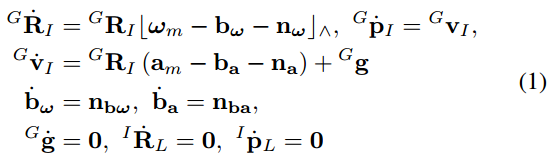 式中,
表示IMU在全局框架中的位置和姿态,
是全局坐标系中的重力矢量,
和
是IMU的测量值,
和
表示
和
的测量噪声,
和
表示
和
驱动下的随机游动过程模型的IMU偏差,符号
^表示一个映射了叉乘运算的向量
的斜对称矩阵。
式中,
表示IMU在全局框架中的位置和姿态,
是全局坐标系中的重力矢量,
和
是IMU的测量值,
和
表示
和
的测量噪声,
和
表示
和
驱动下的随机游动过程模型的IMU偏差,符号
^表示一个映射了叉乘运算的向量
的斜对称矩阵。
设i为IMU测量值的索引。根据FAST-LIO中定义的运算符
,可以在IMU采样周期
处对连续运动学模型(1)进行离散化:  函数f、状态x、输入u和噪声w,定义如下:
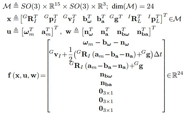
xxxxxxxxxx
// double L_offset_to_I[3] = {0.04165, 0.02326, -0.0284}; // Avia
// vect3 Lidar_offset_to_IMU(L_offset_to_I, 3);
// fast_lio2论文公式(2), 起始这里的f就是将imu的积分方程组成矩阵形式然后再去计算
Eigen::Matrix<double, 24, 1> get_f(state_ikfom &s, const input_ikfom &in)
{
    Eigen::Matrix<double, 24, 1> res = Eigen::Matrix<double, 24, 1>::Zero(); // 将imu积分方程矩阵初始化为0,这里的24个对应了速度(3),角速度(3),外参偏置T(3),外参偏置R(3),加速度(3),角速度偏置(3),加速度偏置(3),位置(3),与论文公式不一致
    vect3 omega;
    in.gyro.boxminus(omega, s.bg); // 得到imu的角速度
    // 加速度转到世界坐标系
    vect3 a_inertial = s.rot * (in.acc - s.ba);
    for (int i = 0; i < 3; i++)
    {
        res(i) = s.vel[i];                       //更新的速度
        res(i + 3) = omega[i];                   //更新的角速度
        res(i + 12) = a_inertial[i] + s.grav[i]; //更新的加速度
    }
    return res;
}
3. df_dx函数和df_dw函数
矩阵
~和
的计算如下(更抽象的推导见论文[55],更具体的推导见论文[22]): 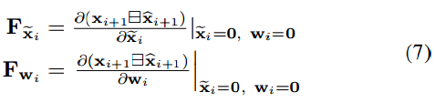 这里以FAT-LIO1的公式作为补充
xxxxxxxxxx
// 对应fast_lio2论文公式(7)
Eigen::Matrix<double, 24, 23> df_dx(state_ikfom &s, const input_ikfom &in)
{
    //当中的23个对应了status的维度计算,为pos(3), rot(3),offset_R_L_I(3),offset_T_L_I(3), vel(3), bg(3), ba(3), grav(2);这一块和fast-lio不同需要注意
    Eigen::Matrix<double, 24, 23> cov = Eigen::Matrix<double, 24, 23>::Zero();
    cov.template block<3, 3>(0, 12) = Eigen::Matrix3d::Identity(); //一开始是一个R3的单位阵,代表速度转移
    vect3 acc_;
    in.acc.boxminus(acc_, s.ba); //拿到加速度
    vect3 omega;
    in.gyro.boxminus(omega, s.bg);                                                //拿到角速度
    cov.template block<3, 3>(12, 3) = -s.rot.toRotationMatrix() * MTK::hat(acc_); //这里的-s.rot.toRotationMatrix()是因为论文中的矩阵是逆时针旋转的
    cov.template block<3, 3>(12, 18) = -s.rot.toRotationMatrix();                 // 将角度转到存入的矩阵中(应该与上面颠倒了)
    Eigen::Matrix<state_ikfom::scalar, 2, 1> vec = Eigen::Matrix<state_ikfom::scalar, 2, 1>::Zero();
    Eigen::Matrix<state_ikfom::scalar, 3, 2> grav_matrix;
    s.S2_Mx(grav_matrix, vec, 21);                                  //将vec的2*1矩阵转为grav_matrix的3*2矩阵
    cov.template block<3, 2>(12, 21) = grav_matrix;                 //存入到矩阵中
    cov.template block<3, 3>(3, 15) = -Eigen::Matrix3d::Identity(); //角速度存入
    return cov;
}
// 对应fast_lio2论文公式(7)
Eigen::Matrix<double, 24, 12> df_dw(state_ikfom &s, const input_ikfom &in)
{
    Eigen::Matrix<double, 24, 12> cov = Eigen::Matrix<double, 24, 12>::Zero();
    cov.template block<3, 3>(12, 3) = -s.rot.toRotationMatrix();   //加速度
    cov.template block<3, 3>(3, 0) = -Eigen::Matrix3d::Identity(); //角速度
    cov.template block<3, 3>(15, 6) = Eigen::Matrix3d::Identity(); //角速度偏置
    cov.template block<3, 3>(18, 9) = Eigen::Matrix3d::Identity(); //加速度偏置
    return cov;
}
4. h_share_model残差计算函数
h_share_model函数主要用来计算残差,并根据IKD-Tree算出可用的点集合,并计算残差。 这里假设在当前迭代更新时状态
的估计值是
,预测状态源于公式(6)中的传播,当k=0 (即第一次迭代前),
。之后,我们将每个测量到的LiDAR点
投影到全局框架,如下 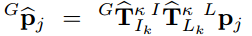 并在ikd-Tree所表示的地图上搜索其最近的5个点。然后利用找到的最接近的相邻点,用测量模型(见(4)和(5))中使用的法向量
和质心
拟合一个局部小平面补丁。此外,用测量方程(5)在
处的一次近似可以得到:
并在ikd-Tree所表示的地图上搜索其最近的5个点。然后利用找到的最接近的相邻点,用测量模型(见(4)和(5))中使用的法向量
和质心
拟合一个局部小平面补丁。此外,用测量方程(5)在
处的一次近似可以得到: 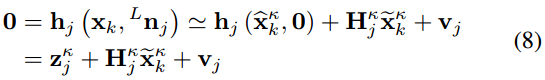 其中,
是
关于
在0处取值的雅可比矩阵;
源于原始测量噪声
;
称为残差:
其中,
是
关于
在0处取值的雅可比矩阵;
源于原始测量噪声
;
称为残差: 
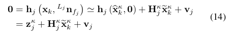
从真值与预测值的等式可推断出,真值与第K次迭代的值的差值,等同于在第K次迭代的时候对误差量进行一阶展开,这里求得的式16是误差的协方差矩阵的先验更新矩阵
xxxxxxxxxx
//计算残差信息
void h_share_model(state_ikfom &s, esekfom::dyn_share_datastruct<double> &ekfom_data)
{
double match_start = omp_get_wtime(); //计算匹配的开始时间
laserCloudOri->clear(); //将body系的有效点云存储清空
corr_normvect->clear(); //将对应的法向量清空
total_residual = 0.0;
/** 最接近曲面搜索和残差计算 **/
#ifdef MP_EN
omp_set_num_threads(MP_PROC_NUM);
#pragma omp parallel for
#endif
//对降采样后的每个特征点进行残差计算
for (int i = 0; i < feats_down_size; i++)
{
PointType &point_body = feats_down_body->points[i]; //获取降采样后的每个特征点
PointType &point_world = feats_down_world->points[i]; //获取降采样后的每个特征点的世界坐标
/* transform to world frame */
//将点转换至世界坐标系下
V3D p_body(point_body.x, point_body.y, point_body.z);
V3D p_global(s.rot * (s.offset_R_L_I * p_body + s.offset_T_L_I) + s.pos); //将点转换至世界坐标系下,从而来计算残差
point_world.x = p_global(0);
point_world.y = p_global(1);
point_world.z = p_global(2);
point_world.intensity = point_body.intensity;
vector<float> pointSearchSqDis(NUM_MATCH_POINTS);
auto &points_near = Nearest_Points[i];
if (ekfom_data.converge) //如果收敛了
{
/** Find the closest surfaces in the map **/
//在已构造的地图上查找特征点的最近邻
ikdtree.Nearest_Search(point_world, NUM_MATCH_POINTS, points_near, pointSearchSqDis);
//如果最近邻的点数小于NUM_MATCH_POINTS或者最近邻的点到特征点的距离大于5m,则认为该点不是有效点
point_selected_surf[i] = points_near.size() < NUM_MATCH_POINTS ? false : pointSearchSqDis[NUM_MATCH_POINTS - 1] > 5 ? false
: true;
}
if (!point_selected_surf[i]) //如果该点不是有效点
continue;
VF(4)
pabcd; //平面点信息
point_selected_surf[i] = false; //将该点设置为无效点,用来计算是否为平面点
//拟合平面方程ax+by+cz+d=0并求解点到平面距离
if (esti_plane(pabcd, points_near, 0.1f)) //找平面点法向量寻找,common_lib.h中的函数
{
float pd2 = pabcd(0) * point_world.x + pabcd(1) * point_world.y + pabcd(2) * point_world.z + pabcd(3); //计算点到平面的距离
float s = 1 - 0.9 * fabs(pd2) / sqrt(p_body.norm()); //计算残差
if (s > 0.9) //如果残差大于阈值,则认为该点是有效点
{
point_selected_surf[i] = true; //再次回复为有效点
normvec->points[i].x = pabcd(0); //将法向量存储至normvec
normvec->points[i].y = pabcd(1);
normvec->points[i].z = pabcd(2);
normvec->points[i].intensity = pd2; //将点到平面的距离存储至normvec的intensit中
res_last[i] = abs(pd2); //将残差存储至res_last
}
}
}
effct_feat_num = 0; //有效特征点数
for (int i = 0; i < feats_down_size; i++)
{
//根据point_selected_surf状态判断哪些点是可用的
if (point_selected_surf[i])
{
// body点存到laserCloudOri中
laserCloudOri->points[effct_feat_num] = feats_down_body->points[i]; //将降采样后的每个特征点存储至laserCloudOri
//拟合平面点存到corr_normvect中
corr_normvect->points[effct_feat_num] = normvec->points[i];
total_residual += res_last[i]; //计算总残差
effct_feat_num++; //有效特征点数加1
}
}
res_mean_last = total_residual / effct_feat_num; //计算残差平均值
match_time += omp_get_wtime() - match_start; //返回从匹配开始时候所经过的时间
double solve_start_ = omp_get_wtime(); //下面是solve求解的时间
// 测量雅可比矩阵H和测量向量的计算 H=J*P*J'
ekfom_data.h_x = MatrixXd::Zero(effct_feat_num, 12); //测量雅可比矩阵H,论文中的23
ekfom_data.h.resize(effct_feat_num); //测量向量h
//求观测值与误差的雅克比矩阵,如论文式14以及式12、13
for (int i = 0; i < effct_feat_num; i++)
{
// 拿到的有效点的坐标
const PointType &laser_p = laserCloudOri->points[i];
V3D point_this_be(laser_p.x, laser_p.y, laser_p.z);
M3D point_be_crossmat; //计算点的叉矩阵
// 从点值转换到叉乘矩阵
point_be_crossmat << SKEW_SYM_MATRX(point_this_be);
// 转换到IMU坐标系下
V3D point_this = s.offset_R_L_I * point_this_be + s.offset_T_L_I; // offset_R_L_I,offset_T_L_I为IMU的旋转姿态和位移,此时转到了IMU坐标系下
M3D point_crossmat;
point_crossmat << SKEW_SYM_MATRX(point_this); //计算imu中点的叉矩阵
// 得到对应的曲面/角的法向量
const PointType &norm_p = corr_normvect->points[i];
V3D norm_vec(norm_p.x, norm_p.y, norm_p.z);
// 计算测量雅可比矩阵H
V3D C(s.rot.conjugate() * norm_vec); //旋转矩阵的转置与法向量相乘得到C
V3D A(point_crossmat * C); //对imu的差距真与C相乘得到A
V3D B(point_be_crossmat * s.offset_R_L_I.conjugate() * C); //对点的差距真与C相乘得到B
ekfom_data.h_x.block<1, 12>(i, 0) << norm_p.x, norm_p.y, norm_p.z, VEC_FROM_ARRAY(A), VEC_FROM_ARRAY(B), VEC_FROM_ARRAY(C);
// 测量:到最近表面/角落的距离
ekfom_data.h(i) = -norm_p.intensity; //点到面的距离
}
solve_time += omp_get_wtime() - solve_start_; //返回从solve开始时候所经过的时间
}
5. 参考链接
https://blog.csdn.net/MWY123_/article/details/124110021 https://zhuanlan.zhihu.com/p/471876531 https://zhuanlan.zhihu.com/p/471876061 https://blog.csdn.net/weixin_42048023/article/details/120515558 https://zhuanlan.zhihu.com/p/476286576


评论(0)
您还未登录,请登录后发表或查看评论