

0. 简介
商场、超市等大多数现实场景的环境随时都在变化。不考虑这些变化的预建地图很容易变得过时。因此,有必要拥有一个最新的环境模型,以促进机器人的长期运行。为此《A General Framework for Lifelong Localization and Mapping in Changing Environment》一文提出了一个通用的全生命周期同步定位和建图 (SLAM) 框架。该框架使用多会话地图表示,并利用有效的地图更新策略,包括地图构建、位姿图细化和稀疏化。为了缓解内存使用量的无限制增加,本文提出了一种基于 Chow-Liu 最大互信息生成树的地图修饰(map-trimming)方法。这篇是高仙的论文,作为商业化基本不可能开源,但是不妨碍我们学习它的思想。
1. 文章贡献
本文提出了一种通用的终身定位和建图框架。具体而言,我们的框架跟踪场景中的变化并维护一个最新的地图,以便准确和鲁棒的定位估计。我们在超市环境中实际运行的商业机器人上测试了我们的方法,连续运行超过一个月。实验结果表明,我们的方法可以在存在显著环境变化的情况下实现准确和鲁棒的定位。
我们的主要贡献总结如下:
- 一个完整的终身SLAM通用框架,可以有效地在变化的环境中操作。
- 一种基于子图的图稀疏化方法,具有恒定的计算和存储复杂度,实现高精度。
- 一个包含激光雷达、IMU和轮式编码器数据的公共数据集,用于变化环境下的终身SLAM。
2. 相关工作
我们由于之前没有介绍过很多Lifelong的SLAM方案,所以这里我们以这篇文章为基础,来熟悉一下相关工作和发展。
A. 终身SLAM
长期运行的机器人需要考虑将环境的变化映射为终身过程:删除旧节点并添加新特征以更新地图[8],[9],[10]和[11]。 Biber等[8]提出了一种动态地图。其关键技术贡献是使用基于样本的表示及其通过稳健统计的解释。在每个定位步骤后更新短期记忆地图,仅在运行后或一天后存储和评估长期地图。 Walcott等[10]提出了动态姿态图SLAM(DPG-SLAM),这是一种算法,旨在通过检测每次通过后的标签更改来删除非活动扫描并将新扫描添加到地图中。但是,由于高计算复杂性,他们维护一个姿态图,其中包含所有扫描节点,这些节点不会实时进行优化。 Ding等[11]提出了一种联合框架,用于车辆定位,该框架自适应地合并来自LiDAR惯性测距和全局匹配模块的结果。为了克服全局匹配的失败,他们还提出了一种环境变化检测方法,以找出何时以及哪个部分的地图应及时更新。
与他们相比,为了降低计算复杂度,我们的方法不包括地图变化检测模块。我们的地图数据结构由多个子地图组成,我们直接替换旧子地图。
B.位姿图稀疏化
生命周期SLAM的另一个任务是在机器人重新访问已经映射的区域时稀疏化位姿图,同时最小化信息损失。计算复杂度和内存使用量应该与探索空间的规模成比例,而不是与定位持续时间成比例。为此,提出了位姿图稀疏化方法。Kretzschmar等人[12]使用期望信息增益作为度量标准,期望信息增益被定义为观测引起的机器人信念不确定性的期望减少量,以减少冗余节点并保持定常大小的位姿图。在[13]中,作者提出了使用Chow-Liu树(CLT) [14]来近似个别消除团结构为稀疏树结构,并寻求最小化信息损失,限制位姿图的大小。Carlevaris等人[14]引入了一种基于因子的通用节点移除方法,在因子图SLAM中称为通用线性约束(GLC)。它在一个被边缘化节点的马尔可夫毯上运作,并计算毯的稀疏近似。在这项工作中,我们将CLT稀疏化方法与子地图裁剪相结合,得出生命周期SLAM流程,如下所示。
3. 方法背景
2描述了本文提出的框架的架构,该系统由三个子系统组成:本地LiDAR测(LLO)、全局LiDAR匹配(GLM)和位姿图细化(PGR)。LLO:构建一系列局部一致的子图。GLM 子系统负责计算传入扫描和全局子图之间的相对约束,以及将子图和约束插入PGR。PGR 是本系统中最重要的部分。它收集来自LLO的子图和来自GLM的约束,修剪旧会话中保存的旧子图,并执行位姿图稀疏化和优化。\ec32e9e49d5143728e2804c6b79f3f4b.png)
3.1 多会话定位
本文的地图更新过程,如图3所示。部署到新环境中的机器人必须执行建图(在会话0中),收集传感器数据(包括LiDAR、IMU和轮式编码器),并构建当前环境的地图。该地图由几个占据栅格子图组成,其中每个子图包括固定数量的LiDAR扫描和相应的位姿,即节点。
两个优点:
-
由于局部扫描到子图匹配,单个子图不受全局优化的影响;
-
通过修饰旧子图并向其添加新子图来更新全局地图很方便。
在建图阶段之后,机器人执行定位任务并从LLO创建新的子图。这些子图总是最新的的,不断记录当前环境的最新特征。一旦创建了新的子图,它就被传输到PGR用于后续的地图更新。除了LLO,传感器数据被输入到GLM。GLM负责计算全局地图中扫描和子地图之间的相对观测约束,并将约束输出给PGR。PGR是本文提出框架的关键子系统,它分别从 LLO和GLM接收最新的子图和约束。PGR由三个模块组成:子图优化、位姿图稀疏化和位姿图优化。它通过替换旧会话中的旧子图来维护最新的子图。
3.2 位姿图优化
3.2.1 子地图修剪
在长时间定位的背景下,每当机器人重新进入之前访问过的地形时,新的子地图就会被添加到全局地图中,而不是旧的子地图。关键思想是修剪旧的子图以限制其数量。大多数现有方法都依赖于环境变化检测。他们需要通过逐个单元地比较旧地图和最新地图来找出何时需要更新定位地图。为了降低计算复杂度,本文计算旧子图的重叠率。如果比率低于定义的阈值,则不会删除旧的子图。否则,它们在下面的位姿图稀疏化模块中被标记为修剪和删除。无论旧子图的状态如何,新子图都会添加到位姿图中。这种方法的优点是可以为在固定区域工作的机器人保持恒定的计算时间。
3.2.2 位姿图稀疏化
本文采用Chow-Liu tree (CLT)方法来对子图进行一个优化,该方法仅可能保证了大量关于位姿图的信息,同时降低了就算复杂度。图4是本文稀疏化的过程。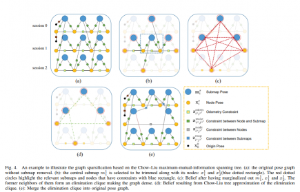
4. 利用CHOW-LIU-TREE(CLT)进行稀疏化
具体的伪代码分为6个步骤,这里参考的是
节点分为以下六类:
- SubmapId& submap_id; 在地图筛选机制中计算出的需要删除的子图id
- std::set
nodes_intra_submap; 上述子图内的所有node id,其与第一步submap_id间constraint的tag为 INTRA_SUBMAP - std::set
node_neighbors; 临近节点,是第二步中nodes_intra_submap中前后各一个与之相连的node - std::set
nodes_inter_sumap; 基于第一步,所有与第一步submap_id间constraint的tag为 INTER_SUBMAP的node - std::set
submaps_inter_node; 基于第二步,所有与第二步nodes_intra_submap间constraint的tag为 INTER_SUBMAP的submap - std::set
submaps_neighbors;
// Algorithom 1,基于input的数据构建一个局部的因子图,获取局部优化后的因子图和包含各个节点信息的完整协方差矩阵或者信息矩阵
ConstructSubFactorGraph(submap_id, nodes_intra_submap, node_neighbors, nodes_inter_sumap, submaps_inter_node, submaps_neighbors, constraints_to_clt)
{
    CONSTRUCT A FACTOR-GRAPH BASED ON GTSAM
}
//Algorithom 2
ChowLiuTreeSparsification(submap_id, nodes_intra_submap, node_neighbors, nodes_inter_sumap, submaps_inter_node, submaps_neighbors, constraints_to_clt, factorgraph)
{
define a priority queue W  (element struct {w, {i,j}} ), ordered by noincreasing w
dense_covariance = Marginalization(submap_id, nodes_intra_submap, node_neighbors, nodes_inter_sumap, submaps_inter_node, submaps_neighbors, factorgraph);
for each edge (i,j) in {node_neighbors, nodes_inter_sumap, submaps_inter_node}
    Compute w = MutualInformation(i, j, dense_covariance);
    W.emplace_back({w,{i,j}});
end for
do MSTKRUSKAL(W, constraints_to_clt, factorgraph, node_neighbors, nodes_inter_sumap, submaps_inter_node);
return constraints;
}
//Algorithom 3
Marginalization(submap_id, nodes_intra_submap, node_neighbors, nodes_inter_sumap, submaps_inter_node, submaps_neighbors, factorgraph)
{
node_to_retain = {node_neighbors, nodes_inter_sumap, submaps_inter_node, submaps_neighbors};
node_to_remove = {submap_id, nodes_intra_submap};
Cov_node_to_retain = factorgraph.jointmarginal(node-to-retain);
Cov_node_to_remove = factorgraph.jointmarginal(node-to-remove);
Cov_retain_remove //完整 graph covariance 中获取,以 node_to_retain为行,node_to_remove为列
dense_covariance = Cov_node_to_retain - Cov_retain_remove*inv(Cov_node_to_remove)*tansport(Cov_retain_remove);
}
//Algorithom 4
MutualInformation(i, j, dense_covariance)
{
cov_ii = dense_covariance(i,i);
cov_ji = dense_covariance(j,i);
cov_jj = dense_covariance(j,j);
result = 0.5 * log2( det(cov_ii)/det(cov_ii - cov_ij*inv(cov_jj)*cov_ji) );
return result;
}
//Algorithom 5
MSTKRUSKAL(W, constraints_to_clt, factorgraph, node_neighbors, nodes_inter_sumap, submaps_inter_node, submaps_neighbors)
{
result_constraints;
for each node i in {node_neighbors, nodes_inter_sumap, submaps_inter_node, submaps_neighbors}
    union_set.insert(i);
for each edge (i,j) in priority queue W in order by poping front
    if (union_set.count(i) != 0 || union_set.count(j) != 0)
        union_set.erase(i);
        union_set.erase(j);
        do ConstraintPairwiseComposition(i, j, constraints_to_clt, factorgraph) to get constraint(i,j);
        result_constraints.emplace_back(constraint(i,j));
return result_constraints;
}
//Algorithom 6
ConstraintPairwiseComposition(i, j, constraints_to_clt, factorgraph)
{
//使用路径联通算法获取pairwise path
//区分纯组合边和混合边,进行计算输出即可
}
下面我们来梳理一下实现 Lifelong Mapping 的思路定期删除 PoseGraph 中冗余节点,在这过程中有两个问题需要考虑:
- 怎么判断并筛选出冗余节点
- 从PoseGraph 中删除冗余节点后,PoseGraph 需要做怎样的调整
4.1 冗余节点的选取
SLAM 的目的是构建周边环境的地图。因此,选取冗余节点的时候主要要考虑的是其对地图的影响:
- 如果去除节点之后对构建的地图不发生变化或变化很小,可以考虑为冗余节点
- 或者冗余节点的数据被其他节点覆盖,这种情况下可以直接删除节点,不会对地图的生成造成影响
了解了冗余节点的定义之后,接下来要来看一下具体怎么进行选择。在 PoseGraph 中每一个节点中都存储了一帧激光数据,以计数构图法为例:地图中每一个栅格(i)都存储被击中的次数hits(i)以及被穿过的次数misses(i)。我们用 hits(i) / (hits(i) + misses(i)) 来表示该栅格是障碍物的概率。在这个背景下,每一个节点中存储该帧激光数据穿过的栅格以及击中的栅格。
在建图中,我们使用全部节点数据构建一个完整的地图 A,得到每一个栅格被击中和被穿过的数据,如下所示: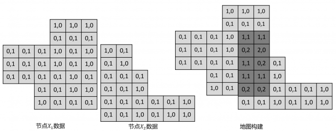
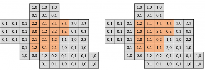
这里注意下,由于在建图过程中位姿已经知道,因此所有节点存储的都是在世界坐标系下的栅格数据。在知道了怎么用节点数据构建图之后,我们需要关注以下,对于一个节点 i,去除一个节点对地图的影响。由上可以知道,我们需要对地图做的变化时,从地图中存储该节点的数据,在该节点穿过的栅格对应的穿过次数减 1,击中的栅格对应的击中次数减 1。如下所示(黄色区域为某一帧激光数据覆盖区域):
从栅格占据概率的考虑出发,我们可以定量分析去除栅格对建图的影响,可以用去除节点前后状态变化的栅格个数作为节点冗余度的指标,如下所示:
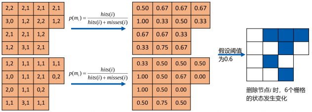
从对地图的影响来看,去除节点状态的状态变化栅格数量越少,意味着该帧数据越冗余,反之亦然。我们选择冗余节点时,以此计算每一个节点的冗余度,并选择其中最冗余的一个节点并且当其冗余度小于一定阈值时将其作为待删除节点。在确定了待删除节点之后,后面两部分我们来讨论以下如何对其进行删除
4.2 PoseGraph 的稠密近似
给定如下例子:
其对应的信息矩阵为:
其中橙色节点为待删除节点,我们将整个图看成一个联合概率分布:
p(x_1, x_2, …, x_9, x_10, x_11)
令:
\begin{aligned}
\alpha &= (x_1, x_2, …, x_8, x_10, x_11) \
\beta &= x
\end{aligned}
则我们要做的是一个边缘化过程,即: p(\alpha, \beta) \rightarrow p(\beta)
根据以下结论,假设我们可以将联合概率分布表示为如下信息向量和信息矩阵表示形式:
p(\alpha, \beta) = N^{-1}(
\begin{bmatrix}
\xi_\alpha \
\xi_\beta
\end{bmatrix},
\begin{bmatrix}
\Omega_{\alpha\alpha} & \Omega_{\alpha\beta} \
\Omega_{\beta\alpha} & \Omega_{\beta\beta}
\end{bmatrix}
)
则其边缘分布也服从高斯分布,p(a) 的信息箱梁和信息矩阵分别如下:
\begin{aligned}
\xi &= \xi_\alpha - \Omega_{\alpha\beta}\Omega^{-1}_{\beta\beta}\xi_{\beta} \
\Omega &= \Omega_{\alpha\alpha} - \Omega_{\alpha\beta}\Omega_{\beta\beta}^{-1}\Omega_{\beta\alpha}
\end{aligned}
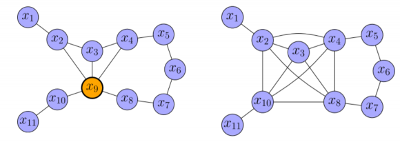
通过这种方法精确边缘化后的 PoseGraph 以及信息矩阵如下所示,待删除节点之间的相邻节点形成一个完整子图,使得图更加稠密。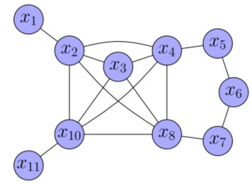

因此我们可以知道,在删除一个节点之后,我们需要在其周边构建一个完全子图,因此需要讨论一下如何计算出完全子图中新增加的边。
这里先引入第一个结论,对完全子图中,假设第 i 个节点和 第 j 个节点相对位姿服从高斯分布:
\begin{aligned}
e_{ij} &\sim N(\mu_{ij}, \Sigma_{ij}) \
\mu_{ij} &= (t_{ij}, \theta_{ij})
\end{aligned}
则第 j 个节点和第 i 个节点相对位姿也服从高斯分布如下:
\begin{aligned}
e_{ji} &\sim N(\mu_{ji}, \Sigma_{ji}) \
\mu_{ji} &= -R\mu_{ij} \
\Sigma_{ji} &= R\Sigma_{ij}R^T \
R &= \begin{bmatrix}
R^T(\theta_{ij}) & 0 \
0 & 1
\end{bmatrix}
\end{aligned}
其中,R(\theta)表示\theta 的旋转矩阵形式
第二个结论:对完全子图中,假设第 i 个节点和 第 j 个节点以及第 j 个节点和第 k 各节点的相对位姿分别服从高斯分布:
\begin{aligned}
e_{ij} &\sim N(\mu_{ij}, \Sigma_{ij}) \
e_{jk} &\sim N(\mu_{jk}, \Sigma_{jk})
\end{aligned}
则第 i 个节点和第 k 个节点的相对位姿也服从高斯分布,参数如下:
\begin{aligned}
e_{ik} &\sim N(\mu_{ik}, \Sigma_{ik}) \
\mu_{ik} &= \mu_{ij} + R\mu_{jk} \
\Sigma_{ik} &= \Sigma_{ij} + R\Sigma_{jk}R^T \
R &= \begin{bmatrix}
R^T(\theta_{ij}) & 0 \
0 & 1
\end{bmatrix}
\end{aligned}
上述两个结论都可以用位姿矩阵转换来证明。
从第二个结论我们可以得出在删除一个节点后如何为其相邻的两个节点构建新的边。除此之外我们还需要考虑一种情况,即这两个和冗余节点相邻的节点本身已经有边时,如何对两边进行融合,这里引入第三个结论:第 i 个节点和第 j 个节点有以下两个相对位姿关系:
\begin{aligned}
e_{ij} &\sim N(\mu_{ij}, \Sigma_{ij}) \
e_{ij}’ &\sim N(\mu_{ij}’, \Sigma_{ij}’)
\end{aligned}
其融合的相对位姿服从以下高斯分布:
\begin{aligned}
e_{ij} &\sim N(\mu_{ij}, \Sigma_{ij}) \
\mu = \Sigma(\Sigma^{-1}_{ij}\mu_{ij} + \Sigma’^{-1}_{ij}\mu_{ij}’) \
\Sigma = (\Sigma_{ij}^{-1} + \Sigma_{ij}’^{-1})^{-1}
\end{aligned}
因此对上述提出的例子中,节点的去除和新边构建过程如下:
4.3 PoseGraph 的稀疏近似
上面我们介绍了 PoseGraph 的稠密近似方法,在上述方法中,每删除一个节点都会在图中构建一个子图,形成很多新的边,因此随着删除节点的数的增加,图会越来越稠密也因此会一定程度上破坏 Hessian 矩阵的稀疏性质,从而无法利用矩阵稀疏性进行快速求解,会很大程度上减慢优化速度。因此这里提出另一种近似方法。
这里先介绍一种近似方法:Chow-Liu Tree 近似,过程如下所示: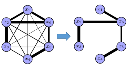
途中边的厚度表示两个变量之间互信息(权重)的大小,这种近似过程等价于最大生成树,数学表示如下:
\begin{aligned}
p(\tilde{\mathbf{x}}) &= p(x_k)\prod_{i=1}^{k-1}p(x_i|x_{i+1}, …, x_k) \
&= p(x_k)\prod_{i=1}^{k-1}p(x_i|x_{i+1}) = q(\tilde{\mathbf{x}})
\end{aligned}
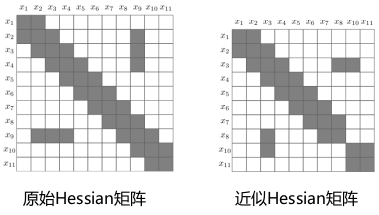
通过稀疏近似之后的 PoseGraph 图以及 Hessian 矩阵如下所示:
5. Chow-LIu Tree
具体代码如下,如果后面有需求会再来开一篇来分析这部分的内容
5.1 ChowLiuTreeApprox.h
#ifndef KARTO_SDK__CHOW_LIU_TREE_APPROX_H_
#define KARTO_SDK__CHOW_LIU_TREE_APPROX_H_

#include <vector>

#include <Eigen/Core>
#include <Eigen/Sparse>

#include "karto_sdk/Karto.h"
#include "karto_sdk/Mapper.h"
#include "karto_sdk/Types.h"

namespace karto
{
  namespace contrib
  {

    /** Marginalizes a variable from a sparse information matrix. */
    Eigen::SparseMatrix<double> ComputeMarginalInformationMatrix(
        const Eigen::SparseMatrix<double> & information_matrix,
        const Eigen::Index discarded_variable_index,
        const Eigen::Index variables_dimension);

    /**
     * Computes a Chow Liu tree approximation to a given pose graph clique.
     *
     * Currently, this function only performs linear approximations to full
     * rank constraints (i.e. constraints with full rank covariance matrices).
     */
    std::vector<Edge<LocalizedRangeScan> *> ComputeChowLiuTreeApproximation(
        const std::vector<Vertex<LocalizedRangeScan> *> & clique,
        const Eigen::MatrixXd & covariance_matrix);

  }  // namespace contrib
}  // namespace karto

#endif // KARTO_SDK__CHOW_LIU_TREE_APPROX_H_
5.2 ChowLiuTreeApprox.cpp
#include "karto_sdk/contrib/ChowLiuTreeApprox.h"
#include "karto_sdk/contrib/EigenExtensions.h"

#include <Eigen/Core>
#include <Eigen/Dense>

#include <boost/graph/adjacency_list.hpp>
#include <boost/graph/kruskal_min_spanning_tree.hpp>

namespace karto
{
  namespace contrib
  {

    Eigen::SparseMatrix<double> ComputeMarginalInformationMatrix(
        const Eigen::SparseMatrix<double> & information_matrix,
        const Eigen::Index discarded_variable_index,
        const Eigen::Index variables_dimension)
    {
      const Eigen::Index dimension = information_matrix.outerSize();
      assert(dimension == information_matrix.innerSize());  // must be square
      const Eigen::Index marginal_dimension = dimension - variables_dimension;
      const Eigen::Index last_variable_index = dimension - variables_dimension;
      // (1) Break up information matrix based on which are the variables
      // kept and which is the variable discarded (vectors `a` and `b` resp.).
      Eigen::SparseMatrix<double>
          information_submatrix_aa, information_submatrix_ab,
          information_submatrix_ba, information_submatrix_bb;
      if (discarded_variable_index == 0) {
        information_submatrix_aa =
            information_matrix.bottomRightCorner(
                marginal_dimension, marginal_dimension);
        information_submatrix_ab =
            information_matrix.bottomLeftCorner(
                marginal_dimension, variables_dimension);
        information_submatrix_ba =
            information_matrix.topRightCorner(
                variables_dimension, marginal_dimension);
        information_submatrix_bb =
            information_matrix.topLeftCorner(
                variables_dimension, variables_dimension);
      } else if (discarded_variable_index == last_variable_index) {
        information_submatrix_aa =
            information_matrix.topLeftCorner(
                marginal_dimension, marginal_dimension);
        information_submatrix_ab =
            information_matrix.topRightCorner(
                marginal_dimension, variables_dimension);
        information_submatrix_ba =
            information_matrix.bottomLeftCorner(
                variables_dimension, marginal_dimension);
        information_submatrix_bb =
            information_matrix.bottomRightCorner(
                variables_dimension, variables_dimension);
      } else {
        const Eigen::Index next_variable_index =
            discarded_variable_index + variables_dimension;
        information_submatrix_aa = StackVertically(
            StackHorizontally(
                information_matrix.topLeftCorner(
                    discarded_variable_index,
                    discarded_variable_index),
                information_matrix.topRightCorner(
                    discarded_variable_index,
                    dimension - next_variable_index)),
            StackHorizontally(
                information_matrix.bottomLeftCorner(
                    dimension - next_variable_index,
                    discarded_variable_index),
                information_matrix.bottomRightCorner(
                    dimension - next_variable_index,
                    dimension - next_variable_index)));
        information_submatrix_ab = StackVertically(
            information_matrix.block(
                0,
                discarded_variable_index,
                discarded_variable_index,
                variables_dimension),
            information_matrix.block(
                next_variable_index,
                discarded_variable_index,
                dimension - next_variable_index,
                variables_dimension));
        information_submatrix_ba = StackHorizontally(
            information_matrix.block(
                discarded_variable_index,
                0,
                variables_dimension,
                discarded_variable_index),
            information_matrix.block(
                discarded_variable_index,
                next_variable_index,
                variables_dimension,
                dimension - next_variable_index));
        information_submatrix_bb =
            information_matrix.block(
                discarded_variable_index,
                discarded_variable_index,
                variables_dimension,
                variables_dimension);
      }

      // (2) Compute generalized Schur's complement over the variables
      // that are kept.
      return (information_submatrix_aa - information_submatrix_ab *
              ComputeGeneralizedInverse(information_submatrix_bb) *
              information_submatrix_ba);
    }

    namespace {

      // An uncertain, gaussian-distributed 2D pose.
      struct UncertainPose2
      {
        Pose2 mean;
        Matrix3 covariance;
      };

      // Returns the target 2D pose relative to the source 2D pose,
      // accounting for their joint distribution covariance.
      UncertainPose2 ComputeRelativePose2(
          const Pose2 & source_pose, const Pose2 & target_pose,
          const Eigen::Matrix<double, 6, 6> & joint_pose_covariance)
      {
        // Computation is carried out as proposed in section 3.2 of:
        //
        //    R. Smith, M. Self and P. Cheeseman, "Estimating uncertain spatial
        //    relationships in robotics," Proceedings. 1987 IEEE International
        //    Conference on Robotics and Automation, 1987, pp. 850-850,
        //    doi: 10.1109/ROBOT.1987.1087846.
        //
        // In particular, this is a case of tail-tail composition of two spatial
        // relationships p_ij and p_ik as in: p_jk = ⊖ p_ij ⊕ p_ik
        UncertainPose2 relative_pose;
        // (1) Compute mean relative pose by simply
        // transforming mean source and target poses.
        Transform source_transform(source_pose);
        relative_pose.mean =
            source_transform.InverseTransformPose(target_pose);
        // (2) Compute relative pose covariance by linearizing
        // the transformation around mean source and target
        // poses.
        Eigen::Matrix<double, 3, 6> transform_jacobian;
        const double x_jk = relative_pose.mean.GetX();
        const double y_jk = relative_pose.mean.GetY();
        const double theta_ij = source_pose.GetHeading();
        transform_jacobian <<
            -cos(theta_ij), -sin(theta_ij),  y_jk,  cos(theta_ij), sin(theta_ij), 0.0,
             sin(theta_ij), -cos(theta_ij), -x_jk, -sin(theta_ij), cos(theta_ij), 0.0,
                       0.0,            0.0,  -1.0,            0.0,           0.0, 1.0;
        const Eigen::Matrix3d covariance =
            transform_jacobian * joint_pose_covariance * transform_jacobian.transpose();
        assert(covariance.isApprox(covariance.transpose()));  // must be symmetric
        assert((covariance.array() > 0.).all());  // must be positive semidefinite
        relative_pose.covariance = Matrix3(covariance);
        return relative_pose;
      }

    }  // namespace

    std::vector<Edge<LocalizedRangeScan> *> ComputeChowLiuTreeApproximation(
        const std::vector<Vertex<LocalizedRangeScan> *> & clique,
        const Eigen::MatrixXd & covariance_matrix)
    {
      // (1) Build clique subgraph, weighting edges by the *negated* mutual
      // information between corresponding variables (so as to apply
      // Kruskal's minimum spanning tree algorithm down below).
      using WeightedGraphT = boost::adjacency_list<
        boost::vecS, boost::vecS, boost::undirectedS, boost::no_property,
        boost::property<boost::edge_weight_t, double>>;
      using VertexDescriptorT =
          boost::graph_traits<WeightedGraphT>::vertex_descriptor;
      WeightedGraphT clique_subgraph(clique.size());
      for (VertexDescriptorT u = 0; u < clique.size() - 1; ++u) {
        for (VertexDescriptorT v = u + 1; v < clique.size(); ++v) {
          const Eigen::Index i = u * 3, j = v * 3;  // need block indices
          const auto covariance_submatrix_ii =
              covariance_matrix.block(i, i, 3, 3);
          const auto covariance_submatrix_ij =
              covariance_matrix.block(i, j, 3, 3);
          const auto covariance_submatrix_ji =
              covariance_matrix.block(j, i, 3, 3);
          const auto covariance_submatrix_jj =
              covariance_matrix.block(j, j, 3, 3);
          const double mutual_information =
              0.5 * std::log2(covariance_submatrix_ii.determinant() / (
                  covariance_submatrix_ii - covariance_submatrix_ij *
                  ComputeGeneralizedInverse(covariance_submatrix_jj) *
                  covariance_submatrix_ji).determinant());
          boost::add_edge(u, v, -mutual_information, clique_subgraph);
        }
      }
      // (2) Find maximum mutual information spanning tree in the clique subgraph
      // (which best approximates the underlying joint probability distribution as
      // proved by Chow & Liu).
      using EdgeDescriptorT =
          boost::graph_traits<WeightedGraphT>::edge_descriptor;
      std::vector<EdgeDescriptorT> minimum_spanning_tree_edges;
      boost::kruskal_minimum_spanning_tree(
          clique_subgraph, std::back_inserter(minimum_spanning_tree_edges));
      // (3) Build tree approximation as an edge list, using the mean and
      // covariance of the marginal joint distribution between each variable
      // to recompute the nonlinear constraint (i.e. a 2D isometry) between them.
      std::vector<Edge<LocalizedRangeScan> *> chow_liu_tree_approximation;
      for (const EdgeDescriptorT & edge_descriptor : minimum_spanning_tree_edges) {
        const VertexDescriptorT u = boost::source(edge_descriptor, clique_subgraph);
        const VertexDescriptorT v = boost::target(edge_descriptor, clique_subgraph);
        auto * edge = new Edge<LocalizedRangeScan>(clique[u], clique[v]);
        const Eigen::Index i = u * 3, j = v * 3;  // need block indices
        Eigen::Matrix<double, 6, 6> joint_pose_covariance_matrix;
        joint_pose_covariance_matrix <<  // marginalized from the larger matrix
            covariance_matrix.block(i, i, 3, 3), covariance_matrix.block(i, j, 3, 3),
            covariance_matrix.block(j, i, 3, 3), covariance_matrix.block(j, j, 3, 3);
        LocalizedRangeScan * source_scan = edge->GetSource()->GetObject();
        LocalizedRangeScan * target_scan = edge->GetTarget()->GetObject();
        const UncertainPose2 relative_pose =
            ComputeRelativePose2(source_scan->GetCorrectedPose(),
                                 target_scan->GetCorrectedPose(),
                                 joint_pose_covariance_matrix);
        // TODO(hidmic): figure out how to handle rank deficient constraints
        assert(relative_pose.covariance.ToEigen().fullPivLu().rank() == 3);
        edge->SetLabel(new LinkInfo(
            source_scan->GetCorrectedPose(),
            target_scan->GetCorrectedPose(),
            relative_pose.mean, relative_pose.covariance));
        chow_liu_tree_approximation.push_back(edge);
      }
      return chow_liu_tree_approximation;
    }

  }  // namespace contrib
}  // namespace karto
5.3 gtest
#include <gtest/gtest.h>

#include <Eigen/Core>
#include <Eigen/Sparse>

#include "karto_sdk/contrib/ChowLiuTreeApprox.h"

namespace
{

using namespace karto;
using namespace karto::contrib;

TEST(ChowLiuTreeApproxTest, Marginalization)
{
  constexpr Eigen::Index block_size = 2;
  Eigen::MatrixXd information_matrix(6, 6);
  information_matrix <<
      1.0, 0.0, 0., 0., 0.5, 0.0,
      0.0, 1.0, 0., 0., 0.0, 0.5,
      0.0, 0.0, 1., 0., 0.0, 0.0,
      0.0, 0.0, 0., 1., 0.0, 0.0,
      0.5, 0.0, 0., 0., 1.0, 0.0,
      0.0, 0.5, 0., 0., 0.0, 1.0;

  Eigen::MatrixXd left_marginal(4, 4);
  left_marginal <<
      0.75, 0.0,  0., 0.,
      0.0,  0.75, 0., 0.,
      0.0,  0.0,  1., 0.,
      0.0,  0.0,  0., 1.;
  constexpr Eigen::Index right_most_block_index = 4;
  EXPECT_TRUE(left_marginal.sparseView().isApprox(
      ComputeMarginalInformationMatrix(
          information_matrix.sparseView(),
          right_most_block_index, block_size)));

  Eigen::MatrixXd right_marginal(4, 4);
  right_marginal <<
      1., 0.,  0.,   0.,
      0., 1.,  0.,   0.,
      0., 0.,  0.75, 0.,
      0., 0.,  0.,   0.75;
  constexpr Eigen::Index left_most_block_index = 0;
  EXPECT_TRUE(right_marginal.sparseView().isApprox(
      ComputeMarginalInformationMatrix(
          information_matrix.sparseView(),
          left_most_block_index, block_size)));

  Eigen::MatrixXd outer_marginal(4, 4);
  outer_marginal <<
      1.0, 0.0, 0.5, 0.0,
      0.0, 1.0, 0.0, 0.5,
      0.5, 0.0, 1.0, 0.0,
      0.0, 0.5, 0.0, 1.0;
  constexpr Eigen::Index inner_block_index = 2;
  EXPECT_TRUE(outer_marginal.sparseView().isApprox(
      ComputeMarginalInformationMatrix(
          information_matrix.sparseView(),
          inner_block_index, block_size)));
}

}  // namespace

int main(int argc, char** argv)
{
  testing::InitGoogleTest(&argc, argv);
  return RUN_ALL_TESTS();
}
6. 参考链接
https://mp.weixin.qq.com/s/LcCsM7Djm1ev2OQ7CODCCQ
https://xiaotaoguo.com/p/lidarslam-lifelong-mapping/
https://zhuanlan.zhihu.com/p/487512031
https://zhuanlan.zhihu.com/p/488778404
https://github.com/SteveMacenski/slam_toolbox/pull/468/files


评论(0)
您还未登录,请登录后发表或查看评论