


本文主要基于以下参考:
[1] John T. Betts. Survey of Numerical Methods for Trajectory Optimization.
[2] Anil V. Rao. A Survey of Numerical Methods For Optimal Control.
[3] John T. Betts. Practical Methods for Optimal Control and Estimation Using Nonlinear Programming 2nd.
[4] A E. Bryson. Applied Optimal Control.
[5] KIRK. Optimal Control Theory: An Introduction.
[6] Matthew Kelly. An Introduction to Trajectory Optimization: How to Do Your Own Direct Collocation.
第一部分
本部分涉及到的内容为[4]中的3.7节部分,考虑到现实中许多问题都比较复杂,比如运载火箭发射,就涉及到火箭一二级分离,这导致了系统动力学在某些时刻发生改变;而运载火箭助推分离又会使火箭质量发生瞬时改变,为了对这种问题进行建模,本节考虑一种更一般性的最优控制问题:
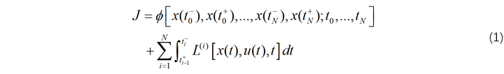
满足约束:


类似于前面,定义:

因此,式(3)的一阶变分如下:
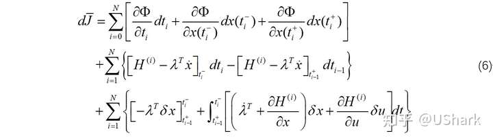
应用下式从式(6)中消去
:

可以得到:
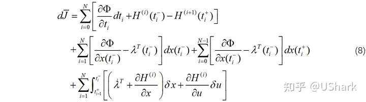
其中,定义

现在根据式(8)可以给出满足的必要条件:

进一步选择时间
满足


第二部分
本部分涉及到的内容为[4]中的3.8节部分,主要涉及到控制变量满足不等式约束,即考虑最优控制问题:

考虑控制变量需要满足不等式约束:

与前面类似,定义哈密顿函数如下:

此时,需要满足的必要条件如下:

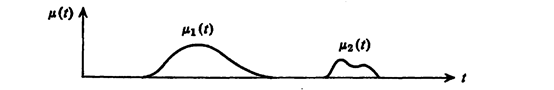
此外,乘子 μ 必须满足:

在求解这类问题中,最优解由约束段和无约束段共同组成,在约束段与无约束段切换处,控制量 u 可能是也可能不是连续的;如果不连续,则该点被称为"corner"。
例题:最小化终端范数。

哈密顿函数定义如下:


其中, C1 和 C2 不可能同时满足,计算最优控制律:

于是,最优控制律可以写作如下:

对上式进一步简化可以得到:

其中,

因此, x(T) 可以从下面的方程中计算得到:

如果求解上式,得到下图所示的控制律:
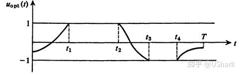
则我们有:

并且可以得到:

首先来看一个例子
比如说对于上述问题:

考虑对上述问题进行求解,参数选择为:

则上述最优控制问题根据前面推导如下:

于是,我们可以写出下述代码来进行求解,假设系统从x0=10 处开始:
%% solve MBVP
global a T
a = 8;
T = 10;

solinit = bvpinit(linspace(0, T, 100), [1 0.5]);

tol = 1E-8;
options = bvpset('RelTol',tol,'AbsTol',[tol tol],'Nmax', 2000);
sol = bvp4c(@MBVPOde, @MBVPbc,solinit,options);

time = sol.x;
state = sol.y(1,:);
costate = sol.y(2,:);

len = length(time);
control = zeros(1,len);
for i=1:len
    control(i) = -Sat(a^2*gg(time(i))*state(end));
end
%% plotting

% state

figure(1); clf
plot(time, state,'r-', 'LineWidth',2)
legend('state','Location','NorthEast')
grid on;

xlabel('Time');ylabel('States')

% costate

figure(2); clf
plot(time, costate,'r-','LineWidth',2)
hold on;
grid on;
xlabel('Time');ylabel('Costates')

% control
figure(3); clf
plot(time, control,'r-', 'LineWidth',2)
hold on;
grid on;

xlabel('Time');ylabel('Control')

%%
function dydt=MBVPOde(t, y, k)
    % y: [x, lambda]
    global a T
    %
    u = -Sat(a^2*gg(t)*y(2)/a^2);
%     if y(2)*gg(t) <= -1
%         u = 1;
%     elseif y(2)*gg(t)>= 1
%         u = -1;
%     else
%         u = -y(2)*gg(t);
%     end

    dydt = [gg(t)*u; 0; ];

end

function res=MBVPbc(ya, yb)
    global a T
    res = [
        ya(1)-10;
        yb(2)-a^2*yb(1)];
end

function ret = gg(t)
    ret = -2*sin(t);
end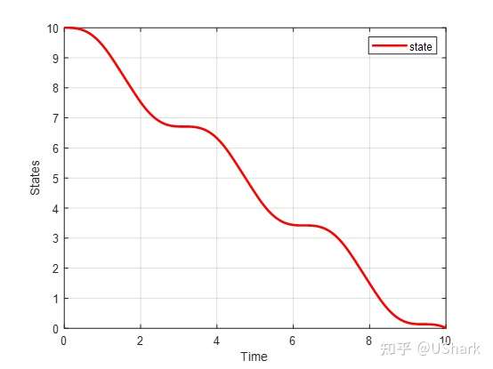
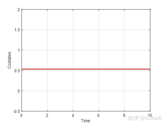
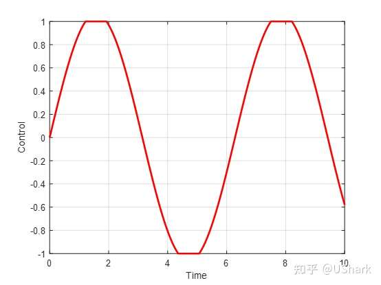
不过由于书中未提供系统的具体参数,因此上述求解过程中采用的参数也是自己试出来的,因此无法保证结果的正确性,仅供参考。
下面再看另外一个例子:

定义哈密顿函数如下:

类似于前面,写出必要条件如下:
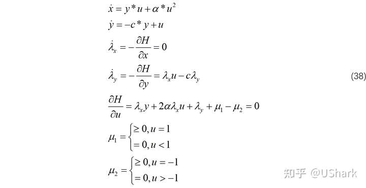
继续对约束进行讨论如下:

此外,边界条件如下:

横截条件如下:

采用代码对该问题进行求解:
% shooting
x0 = [-2.0099; -3.4684; 8.8113];
[x1, feval] = fsolve(@BVPP, x0);
%% 计算控制
y0 = [1;0;x1];
opts = odeset('RelTol',1e-4,'AbsTol',1e-4);
[t, state] = ode45(@BVPOde, [0 1], y0, opts);
npts = length(t);
u = zeros(npts,1);
for i=1:npts
statei = state(i,:);
x=statei(1); y=statei(2);
cx=statei(3); cy=statei(4); tf=statei(5);
alpha = -3/4; c = 1;
mu1 = -cy-cx*y-2*alpha*cx;
type2 = zeros(1,3);
if mu1 >= 0
type2(1) = 1;
end
mu2 = cy+cx*y-2*alpha*cx;
if mu2>= 0
type2(2) = 1;
end
u1 = (-cy-cx*y)/(2*alpha*cx);
if u1>-1 && u1 < 1
type2(3) = 1;
end
if sum(type2) ~= 1
disp('error');
end
if type2(1) == 1
u(i) = 1;
elseif type2(2) == 1
u(i) = -1;
else
u(i) = u1;
end
end
%% plotting
% 状态绘制
figure(1);
plot(t, state(:,1), '-o', t, state(:,2), '-o', t, u, '-o');
grid on;
legend('x','y','u');
%% function definition
function res = BVPP(x)
y0 = [1;0;x];
opts = odeset('RelTol',1e-8,'AbsTol',1e-8);
[t, y] = ode45(@BVPOde, [0 1], y0, opts);
ya = y(1,:);
yb = y(end, :);
res = BVPbc(ya, yb);
end
function dydt=BVPOde(t, state)
x=state(1); y=state(2);
cx=state(3); cy=state(4); tf=state(5);
alpha = -3/4; c = 1;
% 计算控制量u
% type1
mu1 = -cy-cx*y-2*alpha*cx;
type2 = zeros(1,3);
% mu1 >= 0
if mu1 >= 0
type2(1) = 1;
end
mu2 = cy+cx*y-2*alpha*cx;
if mu2>= 0
type2(2) = 1;
end
u1 = (-cy-cx*y)/(2*alpha*cx);
if u1>-1 && u1 < 1
type2(3) = 1;
end
if sum(type2) ~= 1
disp('error');
end
if type2(1) == 1
u = 1;
elseif type2(2) == 1
u = -1;
else
u = u1;
end
dydt= tf*[
y*u+alpha*u^2;
-c*y+u;
0;
-cx*u+c*cy;
0];
end
function res=BVPbc(ya,yb)
x0 = ya(1);
y0 = ya(2);
xf = yb(1);
lamyf=yb(4);
x = yb(1); y=yb(2);
cx = yb(3); cy = yb(4);
alpha = -3/4; c = 1;
mu1 = -cy-cx*y-2*alpha*cx;
type = zeros(1,3);
% mu1 >= 0
if mu1 >= 0
type(1) = 1;
end
mu2 = cy+cx*y-2*alpha*cx;
if mu2>= 0
type(2) = 1;
end
u1 = (-cy-cx*y)/(2*alpha*cx);
if u1>-1 && u1 < 1
type(3) = 1;
end
if sum(type) ~= 1
disp('error');
end
if type(1) == 1
u = 1;
elseif type(2) == 1
u = -1;
else
u = u1;
end
H = cx*(y*u+alpha*u^2)+cy*(-c*y+u)+1;
res = [x0-1;
y0;
xf-2;
lamyf;
H;
];
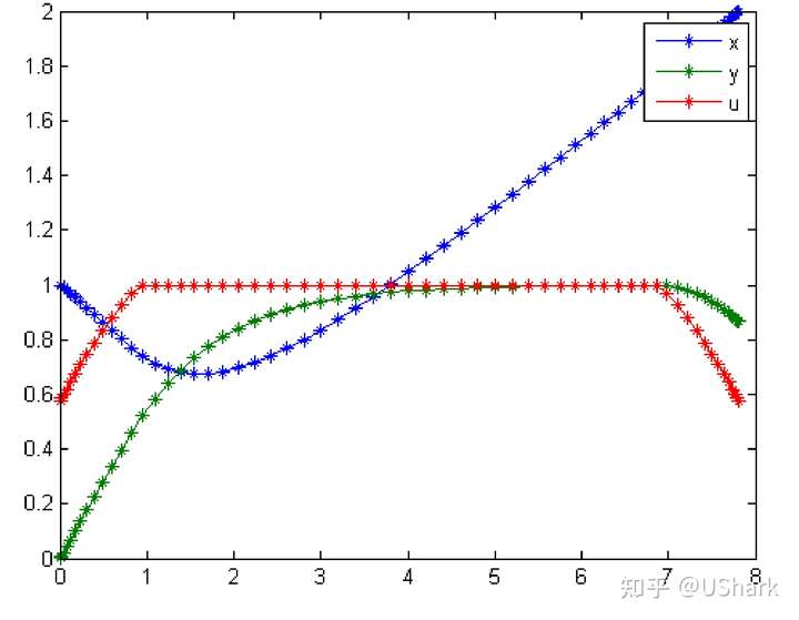
end首先是TOMLAB_PROPT软件给出的求解结果:
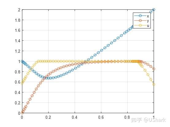
下面给出采用边值方法求解得到的结果:
注:
- 采用bvp4c进行求解时总是无法收敛,不清楚具体是由于什么原因导致的,因此最终采用了打靶法来进行求解。
- 打靶法对于初值比较敏感,尤其是终端时间,因此上述代码的初值是通过直接法首先进行求解得到的结果。


评论(0)
您还未登录,请登录后发表或查看评论