项目场景：

使用matlab中的kmeans命令对数据进行聚类。

问题描述1：

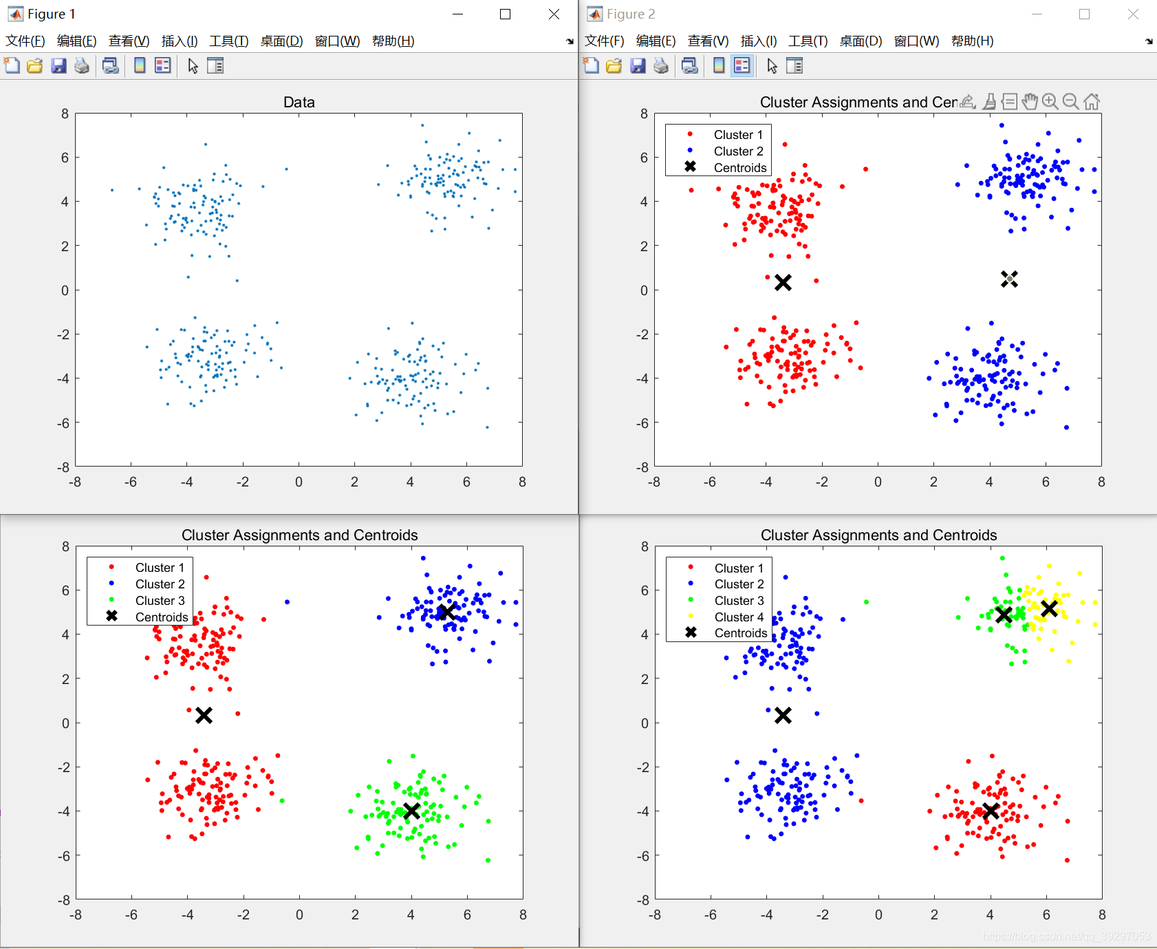
将data1加载到Matlab环境中，并使用“ plot”命令显示数据。 然后通过使用K-means聚类算法（matlab中的“ kmeans”命令），将数据分为2、3和4组，并以不同的颜色显示其中心的聚类数据

命令介绍：

MATLAB函数Kmeans

使用方法：
Idx=Kmeans(X,K)
[Idx,C]=Kmeans(X,K)
[Idx,C,sumD]=Kmeans(X,K)
[Idx,C,sumD,D]=Kmeans(X,K)
[…]=Kmeans(…,’Param1’,Val1,’Param2’,Val2,…)

各输入输出参数介绍：
X: NP的数据矩阵，N为数据个数，P为单个数据维度
K: 表示将X划分为几类，为整数
Idx: N1的向量，存储的是每个点的聚类标号
C: KP的矩阵，存储的是K个聚类质心位置
sumD: 1K的和向量，存储的是类间所有点与该类质心点距离之和
D: N*K的矩阵，存储的是每个点与所有质心的距离

[…]=Kmeans(…,‘Param1’,Val1,‘Param2’,Val2,…)
这其中的参数Param1、Param2等，主要可以设置为如下：

1. ‘Distance’(距离测度)
   ‘sqEuclidean’ 欧式距离（默认时，采用此距离方式）
   ‘cityblock’ 绝度误差和，又称：L1
   ‘cosine’ 针对向量
   ‘correlation’ 针对有时序关系的值
   ‘Hamming’ 只针对二进制数据
2. ‘Start’（初始质心位置选择方法）
   ‘sample’ 从X中随机选取K个质心点
   ‘uniform’ 根据X的分布范围均匀的随机生成K个质心
   ‘cluster’ 初始聚类阶段随机选择10%的X的子样本（此方法初始使用’sample’方法）
   matrix 提供一K*P的矩阵，作为初始质心位置集合
3. ‘Replicates’（聚类重复次数） 整数

解决方案：

matlab代码

load('C:\Users\86177\Desktop\新建文件夹\matlab\data1.mat')
figure;
plot(X(:,1),X(:,2),'.');
title 'Data';

[idx,C] = kmeans(X,2);
C2=C;
figure;
plot(X(idx==1,1),X(idx==1,2),'r.','MarkerSize',12)
hold on
plot(X(idx==2,1),X(idx==2,2),'b.','MarkerSize',12)
plot(C(:,1),C(:,2),'kx',...
     'MarkerSize',15,'LineWidth',3) 
legend('Cluster 1','Cluster 2','Centroids',...
       'Location','NW')
title 'Cluster Assignments and Centroids'
hold off



[idx,C] = kmeans(X,3);
C3=C;
figure;
plot(X(idx==1,1),X(idx==1,2),'r.','MarkerSize',12)
hold on
plot(X(idx==2,1),X(idx==2,2),'b.','MarkerSize',12)
hold on
plot(X(idx==3,1),X(idx==3,2),'g.','MarkerSize',12)
plot(C(:,1),C(:,2),'kx',...
     'MarkerSize',15,'LineWidth',3) 
legend('Cluster 1','Cluster 2','Cluster 3','Centroids',...
       'Location','NW')
title 'Cluster Assignments and Centroids'
hold off



[idx,C] = kmeans(X,4);
C4=C;
figure;
plot(X(idx==1,1),X(idx==1,2),'r.','MarkerSize',12)
hold on
plot(X(idx==2,1),X(idx==2,2),'b.','MarkerSize',12)
hold on
plot(X(idx==3,1),X(idx==3,2),'g.','MarkerSize',12)
hold on
plot(X(idx==4,1),X(idx==4,2),'y.','MarkerSize',12)
plot(C(:,1),C(:,2),'kx',...
     'MarkerSize',15,'LineWidth',3) 
legend('Cluster 1','Cluster 2','Cluster 3','Cluster 4','Centroids',...
       'Location','NW')
title 'Cluster Assignments and Centroids'
hold off

效果展示

问题描述2：

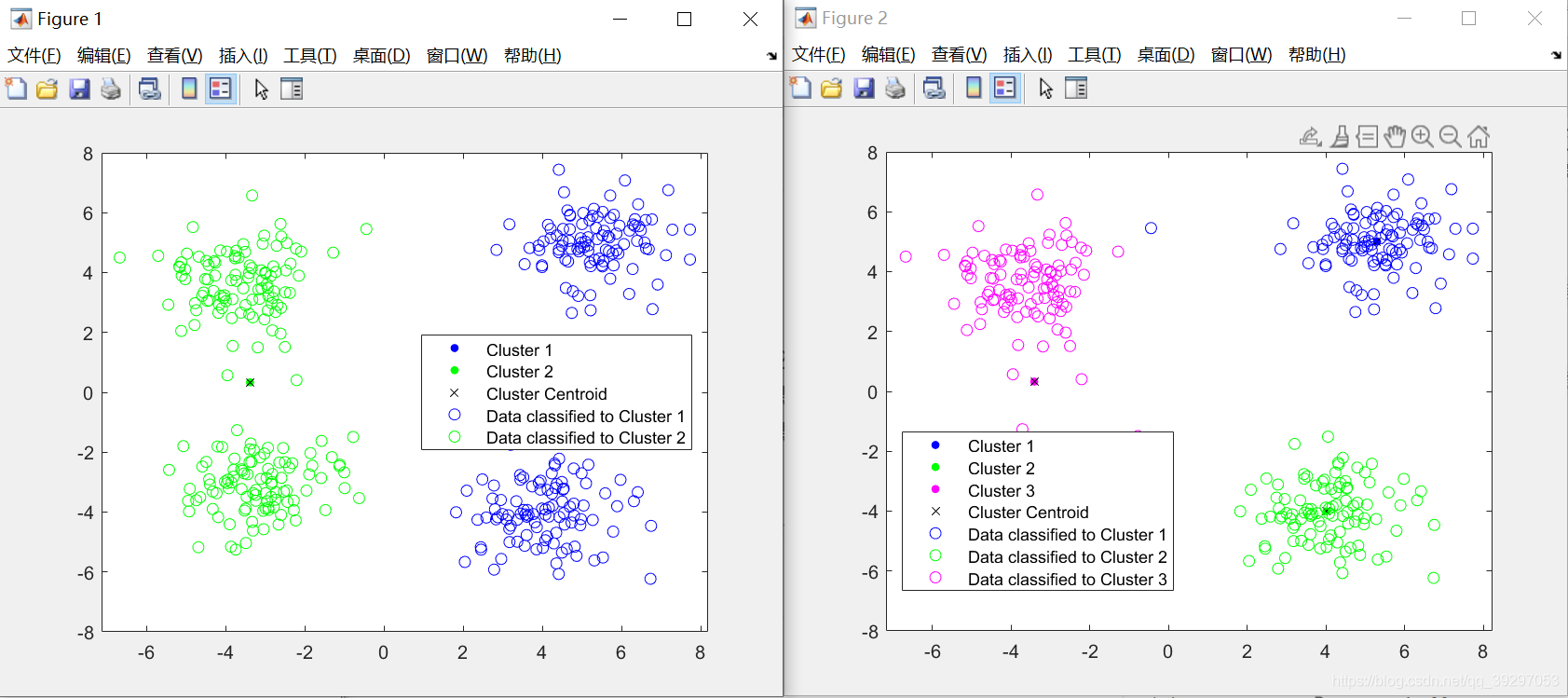
将每个聚类的中心用作训练数据，并对k = 2和3使用KNN算法对上述数据进行分类，并以不同的颜色显示分类的数据。

命令介绍：

MATLAB函数pdist2
1.pdist2(X)
D = pidst(X)主要计算X的行的距离，例如输入X为mn的矩阵，输出D为m(m-1)/2的向量，计算方法如下例子：

X=[1,2;3,4;5,1] 3*2的矩阵;

pdist(X)计算结果为[2.8284,4.1231,3.6056];

计算方法为第二行与第一行距离(3-1)(3-1)+(4-2)(4-2)得到的结果开平方为2.8284，第三行与第一行距离(5-1)(5-1)+(1-2)(1-2)得到的结果开平方为4.1231，第三行与第二行距离(5-3)(5-3)+(1-4)(1-4)得到的结果开平方为3.6056.

2.pdist(X, Y)
X为ab矩阵，Y为cb矩阵，矩阵的每一行代表一个元素，返回一个a*c矩阵，代表X，Y任意两个元素之间的距离。

解决方案：

matlab代码（接上部分）

[idx,C] = kmeans(C2,2);
figure
gscatter(C2(:,1),C2(:,2),idx,'bgm')
hold on
plot(C(:,1),C(:,2),'kx')
legend('Cluster 1','Cluster 2','Cluster Centroid')
Xtest =X;
[~,idx_test] = pdist2(C,Xtest,'euclidean','Smallest',1);
gscatter(Xtest(:,1),Xtest(:,2),idx_test,'bgm','ooo')
legend('Cluster 1','Cluster 2','Cluster Centroid', ...
    'Data classified to Cluster 1','Data classified to Cluster 2' )
%**************************************************
[idx,C] = kmeans(C3,3);
figure
gscatter(C3(:,1),C3(:,2),idx,'bgm')
hold on
plot(C(:,1),C(:,2),'kx')
legend('Cluster 1','Cluster 2','Cluster 3','Cluster Centroid')
Xtest =X;
[~,idx_test] = pdist2(C,Xtest,'euclidean','Smallest',1);
gscatter(Xtest(:,1),Xtest(:,2),idx_test,'bgm','ooo')
legend('Cluster 1','Cluster 2','Cluster 3','Cluster Centroid', ...
    'Data classified to Cluster 1','Data classified to Cluster 2', ...
    'Data classified to Cluster 3')

效果展示