

默认加载以下模块:
import os
import json
from PIL import Image
import matplotlib.pyplot as plt
import numpy as np

import torch
import torch.nn as nn
import torch.nn.functional as F
from torch import optim
import torchvision
from torchvision import models
from torch.utils.data import Dataset
from torchvision import transforms
from torch.utils.data import DataLoader
import visdom
# from tensorboardX import SummaryWriter
from torch.utils.tensorboard import SummaryWriter
微调 Fine-Tuning
假设我们想从图像中识别出不同种类的椅子,然后将购买链接推荐给用户。一种可能的方法是先找出 100 种常见的椅子,为每种椅子拍摄 1,000 张不同角度的图像,然后在收集到的图像数据集上训练一个分类模型。这个椅子数据集虽然可能比 Fashion-MNIST 数据集要庞大,但样本数仍然不及 ImageNet 数据集中样本数的十分之一。这可能会导致适用于 ImageNet 数据集的复杂模型在这个椅子数据集上过拟合。同时,因为数据量有限,最终训练得到的模型的精度也可能达不到实用的要求。为了应对上述问题,一个显而易见的解决办法是收集更多的数据。然而,收集和标注数据会花费大量的时间和资金。另外一种解决办法是应用迁移学习,将从源数据集学到的知识迁移到目标数据集上
下面介绍迁移学习中的一种常用技术:微调,微调由以下 4 步构成:
(1) 在源数据集(如 ImageNet 数据集)上预训练一个神经网络模型,即源模型
(2) 创建一个新的神经网络模型,即目标模型。它复制了源模型上除了输出层外的所有模型设计及其参数。我们假设这些模型参数包含了源数据集上学习到的知识,且这些知识同样适用于目标数据集。我们还假设源模型的输出层与源数据集的标签紧密相关,因此在目标模型中不予采用
(3) 为目标模型添加一个输出大小为目标数据集类别个数的输出层,并随机初始化该层的模型参数
(4) 在目标数据集(如椅子数据集)上训练目标模型。我们将从头训练输出层,而其余层的参数都是基于源模型的参数微调得到的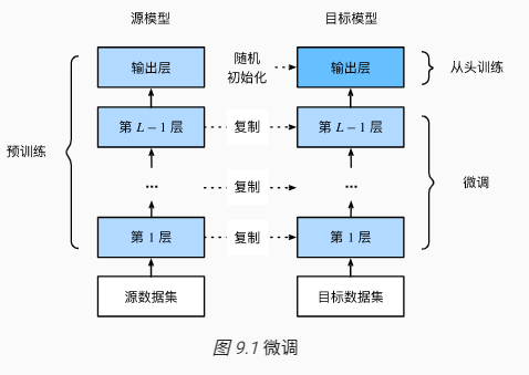
获取 PyTorch 预训练模型
获取模型
- You can construct a model with random weights by calling its constructor:
resnet18 = models.resnet18()
alexnet = models.alexnet()
vgg16 = models.vgg16()
squeezenet = models.squeezenet1_0()
densenet = models.densenet161()
inception = models.inception_v3()
googlenet = models.googlenet()
shufflenet = models.shufflenet_v2_x1_0()
mobilenet = models.mobilenet_v2()
resnext50_32x4d = models.resnext50_32x4d()
wide_resnet50_2 = models.wide_resnet50_2()
mnasnet = models.mnasnet1_0()
获取预训练模型
- We provide pre-trained models. hese can be constructed by passing
pretrained=True: -
resnet18 = models.resnet18(pretrained=True) alexnet = models.alexnet(pretrained=True) squeezenet = models.squeezenet1_0(pretrained=True) vgg16 = models.vgg16(pretrained=True) densenet = models.densenet161(pretrained=True) inception = models.inception_v3(pretrained=True) googlenet = models.googlenet(pretrained=True) shufflenet = models.shufflenet_v2_x1_0(pretrained=True) mobilenet = models.mobilenet_v2(pretrained=True) resnext50_32x4d = models.resnext50_32x4d(pretrained=True) wide_resnet50_2 = models.wide_resnet50_2(pretrained=True) mnasnet = models.mnasnet1_0(pretrained=True) - 更改权重下载文件夹: Instancing a pre-trained model will download its weights to a cache directory. This directory can be set using the TORCH_MODEL_ZOO environment variable. See torch.utils.model_zoo.load_url() for details.
训练、预测的不同模式: Some models use modules which have different training and evaluation behavior, such as batch normalization. To switch between these modes, use model.train() or model.eval() as appropriate.
对输入图像进行标准化: All pre-trained models expect input images normalized in the same way, i.e. mini-batches of 3-channel RGB images of shape ( 3 × H × W ) (3 \times H \times W)(3×H×W), where H HH and W WW are expected to be at least 224. The images have to be loaded in to a range of [ 0 , 1 ] [0, 1][0,1] and then normalized using mean = [0.485, 0.456, 0.406] and std = [0.229, 0.224, 0.225].
关于为什么标准化使用 mean = [0.485, 0.456, 0.406] and std = [0.229, 0.224, 0.225]?文档中给了这个解释,下面截取一些有用信息:The origin of the mean=[0.485, 0.456, 0.406] and std=[0.229, 0.224, 0.225] we use for the normalization transforms on almost every model is only partially known. We know that they were calculated them on a random subset of the train split of the ImageNet2012 dataset. Which images were used or even the sample size as well as the used transformation are unfortunately lost. I’ve tried to reproduce them and found that we probably resized each image to 256 and center cropped it to 224 afterwards. The process for obtaining the values of mean and std is roughly equivalent to:
import torch
from torchvision import datasets, transforms as T

transform = T.Compose([T.Resize(256), T.CenterCrop(224), T.ToTensor()])
dataset = datasets.ImageNet(".", split="train", transform=transform)

means = []
stds = []
for img in subset(dataset):
    means.append(torch.mean(img))
    stds.append(torch.std(img))

mean = torch.mean(torch.tensor(means))
std = torch.mean(torch.tensor(stds))
AlexNet
models.alexnet(pretrained=False, progress=True, **kwargs)
progress(bool) – IfTrue, displays a progress bar of the download to stderr
VGG
models.vgg16_bn(pretrained=False, progress=True, **kwargs)
ResNet
models.resnet18(pretrained=False, progress=True, **kwargs)
DenseNet
models.densenet169(pretrained=False, progress=True, **kwargs)
Inception v3
models.inception_v3(pretrained=False, progress=True, **kwargs)
Important: In contrast to the other models the inception_v3 expects tensors with a size of N × 3 × 299 × 299 N \times 3 \times 299 \times 299N×3×299×299, so ensure your images are sized accordingly.
aux_logits(bool) – IfTrue, add an auxiliary branch that can improve training.Default:Truetransform_input(bool) – IfTrue, preprocesses the input according to the method with which it was trained on ImageNet.Default:False
This requires scipy to be installed
GoogLeNet (Inception v1)
models.googlenet(pretrained=False, progress=True, **kwargs)
aux_logits(bool) – IfTrue, add an auxiliary branch that can improve training.Default:Truetransform_input(bool) – IfTrue, preprocesses the input according to the method with which it was trained on ImageNet.Default:False
This requires scipy to be installed
利用迁移学习进行热狗识别
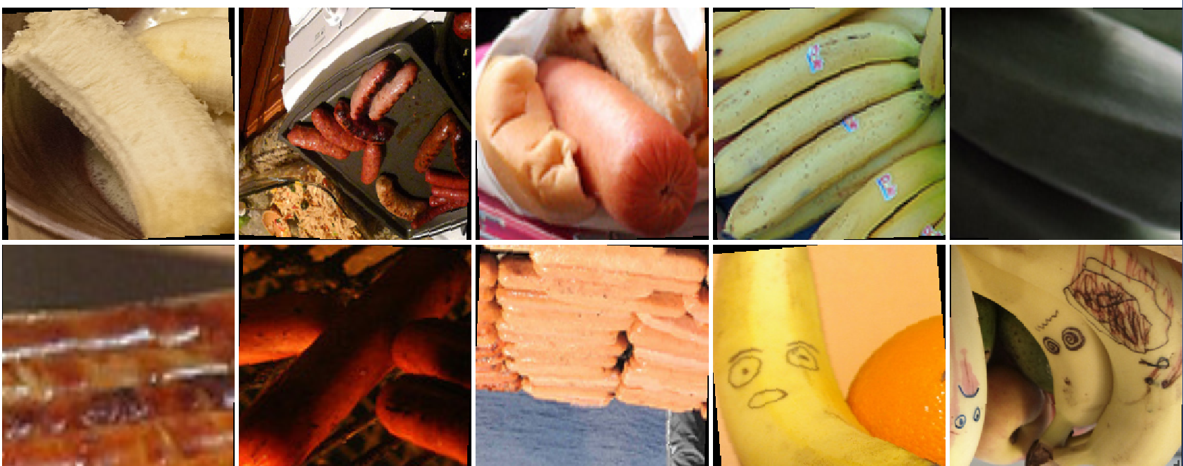
我们使用的热狗数据集是从网上抓取的,它含有 1400 张包含热狗的正类图像,和同样多包含其他食品的负类图像。各类的 1000 张图像被用于训练,其余则用于测试。数据集下载链接:https://apache-mxnet.s3-accelerate.amazonaws.com/gluon/dataset/hotdog.zip。
将下载好的数据集解压,得到两个文件夹 hotdog/train 和 hotdog/test。这两个文件夹下面均有 hotdog/train 和 hotdog/test两个类别文件夹,每个类别文件夹里面是图像文件
在训练时,我们先从图像中裁剪出随机大小和随机高宽比的一块随机区域,然后将该区域缩放为高和宽均为 224 像素的输入。测试时,我们将图像的高和宽均缩放为 256 像素,然后从中裁剪出高和宽均为 224 像素的中心区域作为输入。此外,我们对 RGB 三个颜色通道的数值做标准化:每个数值减去该通道所有数值的平均值,再除以该通道所有数值的标准差作为输出
加载数据集
class HotdogData(Dataset):
    def __init__(self, img_path, transforms=None):
        # 初始化,读取数据集
        self.transforms = transforms
        self.img_path = img_path
        self.pos_dir = img_path + '/hotdog'
        self.neg_dir = img_path + '/not-hotdog'
        self.pos_num = len(os.listdir(self.pos_dir))
        self.neg_num = len(os.listdir(self.neg_dir))

    def __len__(self):
        return self.pos_num + self.neg_num

    def __getitem__(self, index):
        if index < self.pos_num: # 获取正样本
            label = 1
            img = Image.open(self.pos_dir + '/' + str(index if self.img_path[-5:] == 'train' else index + 1000) + '.png')
        else: # 获取负样本
            label = 0
            img = Image.open(self.neg_dir + '/' + str((index - self.pos_num) if self.img_path[-5:] == 'train' else index - self.pos_num + 1000) + '.png')

        if self.transforms:
            img = self.transforms(img)

        return img, label
train_transform = transforms.Compose([
                    transforms.RandomResizedCrop(size=224, scale=(0.8, 1.0)), # 将图像随意裁剪,宽高均为224
                    transforms.RandomHorizontalFlip(), # 以 0.5 的概率左右翻转图像
                    transforms.RandomVerticalFlip(),
#                     transforms.ColorJitter(brightness=0.5, contrast=0.5, saturation=0.5, hue=0),
                    transforms.RandomRotation(degrees=5, expand=False, fill=None),
                    transforms.ToTensor(), # 将 PIL 图像转为 Tensor,并且进行归一化
                    transforms.Normalize([0.485, 0.456, 0.406], [0.229, 0.224, 0.225]) # 标准化
                ])
test_transform = transforms.Compose([
                    transforms.Resize(256),
                    transforms.CenterCrop(224),
                    transforms.ToTensor(), # 将 PIL 图像转为 Tensor,并且进行归一化
                    transforms.Normalize([0.485, 0.456, 0.406], [0.229, 0.224, 0.225]) # 标准化
                ])

train_data = HotdogData('D:/Download/Dataset/hotdog/train', transforms=train_transform)
trainloader = DataLoader(train_data, batch_size=64, shuffle=True)

test_data = HotdogData('D:/Download/Dataset/hotdog/test', transforms=test_transform)
testloader = DataLoader(test_data, batch_size=64, shuffle=True)
可视化图片:
# get some random training images
dataiter = iter(trainloader)
images, labels = dataiter.next() # 选取十张
images = images[:10]
labels = labels[:10]

# show images
vis = visdom.Visdom(env='hotdog')
# images = images / 2 + 0.5     # unnormalize
vis.images(images, nrow=5, opts=dict(title='hotdog'))
# print labels
print(' '.join('%d' % label for label in labels))
定义和初始化模型
使用在 ImageNet 数据集上预训练的 ResNet-18 作为源模型
device = torch.device("cuda:0" if torch.cuda.is_available() else "cpu")

net = models.resnet18(pretrained=True, progress=True)
net = net.to(device)
可视化网络结构:
# 可视化网络结构
dummy_input = torch.rand(13, 3, 224, 224)
with SummaryWriter('runs/exp-1') as w:
    w.add_graph(net, (dummy_input,))

可以看到,预训练模型最后的全连接层输出的类别为 1000 个:
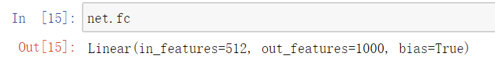
由于现在要处理二分类问题,因此需要修改一下全连接层,将上面的代码修改成如下形式:
device = torch.device("cuda:0" if torch.cuda.is_available() else "cpu")

net = models.resnet18(pretrained=True, progress=True)
net = net.to(device)

# 全连接层的输入通道in_channels个数
num_fc_in = net.fc.in_features

# 改变全连接层,2分类问题,out_features = 2
net.fc = nn.Linear(num_fc_in, 2)
定义损失函数层:
criterion = nn.CrossEntropyLoss()
- 由于全连接层前面层的参数是在 ImageNet 数据集上预训练得到的,已经足够好,因此一般只需使用较小的学习率来微调这些参数。而全连接层参数采用了随机初始化,一般需要更大的学习率从头训练。可以将全连接层的学习率设为其他层学习率的十倍,也可以设置前面的几个卷积层不进行学习
-
lr = 0.001 / 10 fc_params = list(map(id, net.fc.parameters())) # 取得全连接层的参数内存地址的列表 base_params = filter(lambda p: id(p) not in fc_params, net.parameters()) # 取得其他层参数的列表 optimizer = optim.Adam([ {'params': base_params}, {'params': net.fc.parameters(), 'lr': lr * 10}], lr=lr, betas=(0.9, 0.999)) -
训练模型
epoch_num = 2 evaluate_batch_num = 5 for epoch in range(epoch_num): # loop over the dataset multiple times running_loss = 0.0 epoch_loss = 0.0 for i, data in enumerate(trainloader): # get the inputs inputs, labels = data # zero the parameter gradients optimizer.zero_grad() # forward + backward + optimize outputs = net(inputs) loss = criterion(outputs, labels) loss.backward() optimizer.step() # print statistics running_loss += loss.item() epoch_loss += loss.item() if i % evaluate_batch_num == evaluate_batch_num - 1: # print every 2000 mini-batches print('[%d, %5d] loss: %.3f' % (epoch, i + 1, running_loss / evaluate_batch_num)) with SummaryWriter('runs/exp-1') as w: w.add_scalar('TrainLoss/epoch' + str(epoch), running_loss / evaluate_batch_num, i // evaluate_batch_num) running_loss = 0.0 with SummaryWriter('runs/exp-1') as w: w.add_scalar('TrainLoss/all', epoch_loss / len(trainloader), epoch) epoch_loss = 0.0 print('Finished Training') -
[0, 5] loss: 0.536 [0, 10] loss: 0.225 [0, 15] loss: 0.208 [0, 20] loss: 0.132 [0, 25] loss: 0.158 [0, 30] loss: 0.249 [1, 5] loss: 0.084 [1, 10] loss: 0.093 [1, 15] loss: 0.100 [1, 20] loss: 0.101 [1, 25] loss: 0.084 [1, 30] loss: 0.089 Finished Training 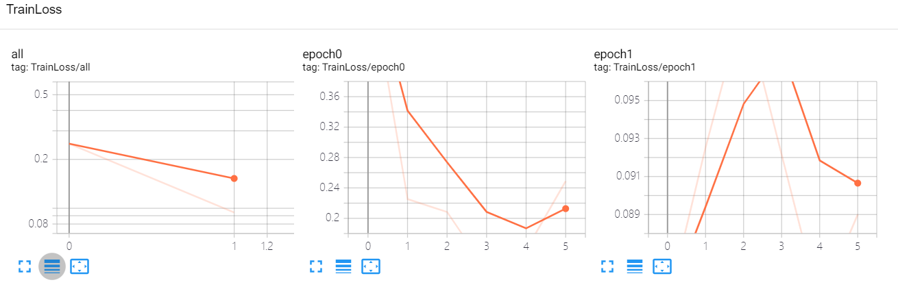
测试模型
correct = 0
total = 0
with torch.no_grad():
    for data in testloader:
        images, labels = data
        outputs = net(images)
        _, predicted = torch.max(outputs.data, 1)
        total += labels.size(0)
        correct += (predicted == labels).sum().item()

print('Accuracy of the network on the test images: %d %%' % (
    100 * correct / total))
Accuracy of the network on the test images: 93 %
- 可以看到,在运用了迁移学习之后,仅训练了两个 epoch,精度就达到了 93%
参考文献
- PyTorch 官方教程中文版
- Pytorch 中文文档
- PyTorch英文文档
- 《深度学习之 PyTorch 物体检测实战》
- 《动手学深度学习》


评论(0)
您还未登录,请登录后发表或查看评论