问题说明

ceres-solver库是google的非线性优化库，可以对slam问题，机器人位姿进行优化，使其建图的效果得到改善。pose_graph_3d是官方给出的二维平面上机器人位姿优化问题，需要读取一个g2o文件，运行程序后返回一个poses_original.txt和一个poses_optimized.txt，大家按字面意思理解，内部格式长这样：

pose_id x y z q_x q_y q_z q_w
pose_id x y z q_x q_y q_z q_w
pose_id x y z q_x q_y q_z q_w
...

按examples中pose_graph_3d包内的README操作。)得到这两个文件后，用官方提供的plot_results.py可以画出原始和优化后的位姿地图，类似下图：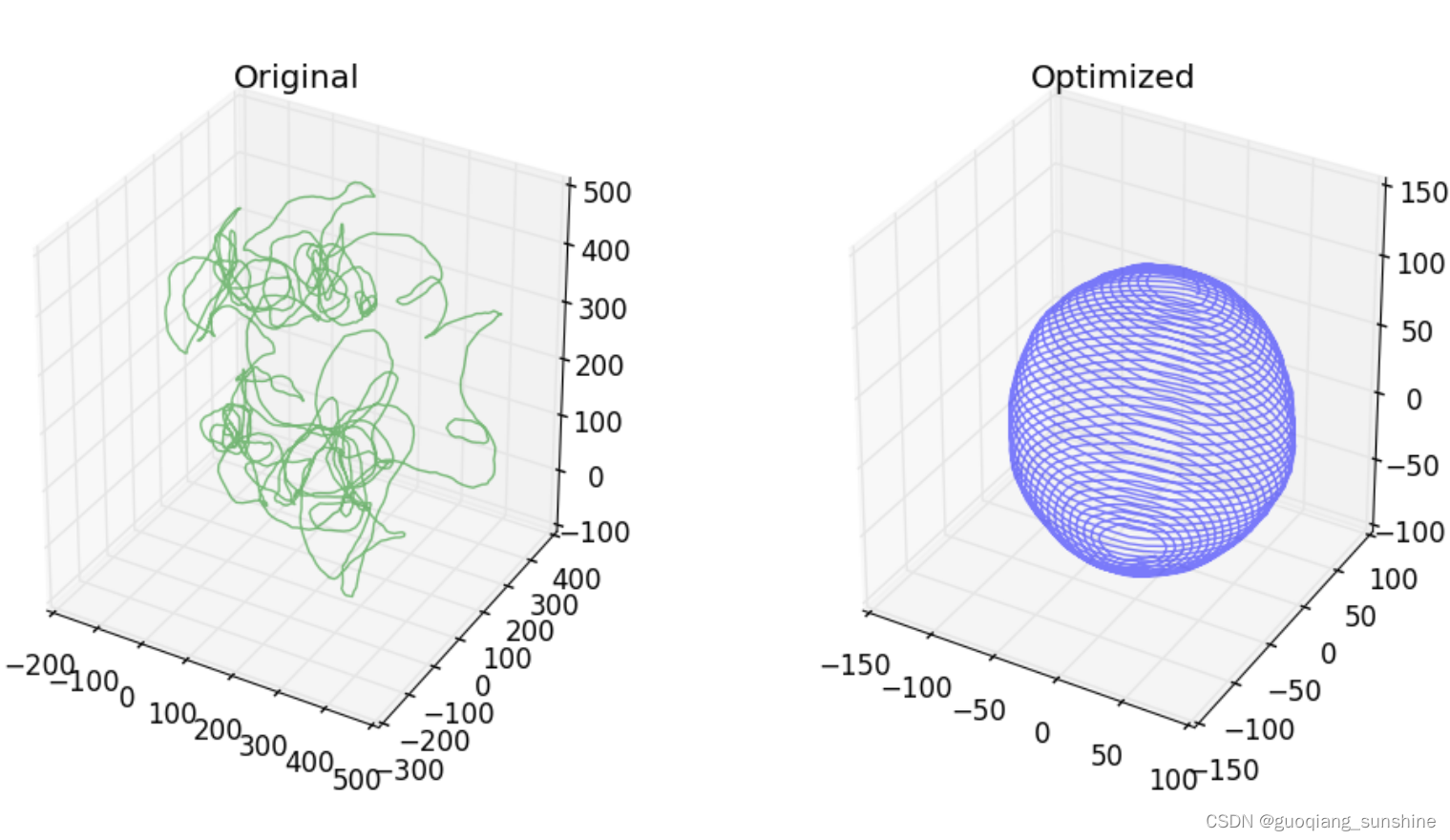

变量说明

重要变量为以下几个：
constraints：vector，例程中起名叫VectorOfConstraints，放入变量的类型为Constraint3d， 如下所示，注意eigen的对齐。

//eigen 对齐，可能是因为Constraint3d里面有eigen的数据类型
typedef std::vector<Constraint3d, Eigen::aligned_allocator<Constraint3d> >
    VectorOfConstraints;

含义为机器人两个pose之间的限制，Constraint3d包括两个pose的id，相对旋转矩阵t_be(含义为从e帧变换到b帧的变换矩阵)，和协方差阵。constraints这个变量描述的是观测量测量量measurement，即机器人认为自己感知到的正确的数据。

poses: map类指针，例程起名为MapOfPoses键值对为id和 Pose3d ，后面两个参数为按键从小到大排列和eigen的内部对齐。如下所示。

//map的四个参数 键是整形，值是Pose3d，按key值从小到大排序，(Pose3d含有eigen的数据类型)需要对齐
typedef std::map<int, Pose3d, std::less<int>,
                 Eigen::aligned_allocator<std::pair<const int, Pose3d> > >
    MapOfPoses;

此步搭建了costfunction，详情下面介绍。

//为四元数添加一个LocalParameterization，定义新的求导方式,求解雅可比矩阵
//定义一个父类指针指向子类
  ceres::LocalParameterization* quaternion_local_parameterization =
      new EigenQuaternionParameterization;

此步new了一个LocalParameterization，详情下面介绍。

Costfunction的搭建

使用ceres库的关键是构造 costfunction ，ceres官方搭建的costfunction，同样有一个类表示，名为PoseGraph3dErrorTerm，具体如下所示：

class PoseGraph3dErrorTerm {
 public:
  PoseGraph3dErrorTerm(const Pose3d& t_ab_measured,
                       const Eigen::Matrix<double, 6, 6>& sqrt_information)
      : t_ab_measured_(t_ab_measured), sqrt_information_(sqrt_information) {}

  template <typename T>
  bool operator()(const T* const p_a_ptr, const T* const q_a_ptr,
                  const T* const p_b_ptr, const T* const q_b_ptr,
                  T* residuals_ptr) const {
    Eigen::Map<const Eigen::Matrix<T, 3, 1> > p_a(p_a_ptr);
    Eigen::Map<const Eigen::Quaternion<T> > q_a(q_a_ptr);

    Eigen::Map<const Eigen::Matrix<T, 3, 1> > p_b(p_b_ptr);
    Eigen::Map<const Eigen::Quaternion<T> > q_b(q_b_ptr);

    // Compute the relative transformation between the two frames.
    Eigen::Quaternion<T> q_a_inverse = q_a.conjugate();
    Eigen::Quaternion<T> q_ab_estimated = q_a_inverse * q_b;

    // Represent the displacement between the two frames in the A frame.
    Eigen::Matrix<T, 3, 1> p_ab_estimated = q_a_inverse * (p_b - p_a);

    // Compute the error between the two orientation estimates.
    Eigen::Quaternion<T> delta_q =
        t_ab_measured_.q.template cast<T>() * q_ab_estimated.conjugate();

    // Compute the residuals.
    // [ position         ]   [ delta_p          ]
    // [ orientation (3x1)] = [ 2 * delta_q(0:2) ]
    Eigen::Map<Eigen::Matrix<T, 6, 1> > residuals(residuals_ptr);
    residuals.template block<3, 1>(0, 0) =
        p_ab_estimated - t_ab_measured_.p.template cast<T>();
    residuals.template block<3, 1>(3, 0) = T(2.0) * delta_q.vec();

    // Scale the residuals by the measurement uncertainty.
    residuals.applyOnTheLeft(sqrt_information_.template cast<T>());

    return true;
  }

  static ceres::CostFunction* Create(
      const Pose3d& t_ab_measured,
      const Eigen::Matrix<double, 6, 6>& sqrt_information) {
    return new ceres::AutoDiffCostFunction<PoseGraph3dErrorTerm, 6, 3, 4, 3, 4>(
        new PoseGraph3dErrorTerm(t_ab_measured, sqrt_information));
  }

  EIGEN_MAKE_ALIGNED_OPERATOR_NEW

 private:
  // The measurement for the position of B relative to A in the A frame.
  const Pose3d t_ab_measured_;
  // The square root of the measurement information matrix.
  const Eigen::Matrix<double, 6, 6> sqrt_information_;
};

其中包括：
一个构造函数PoseGraph3dErrorTerm( t_ab_measured,sqrt_information )；
一个运算符重载operator()( p_a_ptr, q_a_ptr, p_b_ptr, q_b_ptr, residuals_ptr )，其中residuals_ptr指向的东西是计算出的残差；
一个构造costfunction的函数Create( t_ab_measured, sqrt_information )。

operator()的作用
传入参数计算残差，残差有六维，如下所示：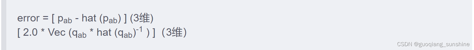

其中Vec()函数取四元数的虚部，也就是跟旋转向量相关的那部分，这样的话最小化误差的理想状态最后三维会是0向量。pab 是a坐标系中表示的机器人在b时的位置，qab是b到a的旋转四元数， 由下式计算。带hat的是测量值，是在时刻a时机器人坐标系下观察的测量值。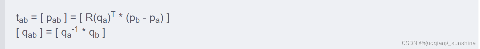

pb 和 pa 的定义见pose_graph_2d里的说明。 qab是由 b→world→a 得到。

代码中首先将传入的参数map到eigen的数据类型，p_a和p_b(Eigen::Matrix)，q_a和q_b(Eigen::Quaternion)，关于eigen的map问题可点击这里，然后将q_a取了其共轭(conjugate)，并当做其逆使用，这里有些不懂它为什么这么做，inverse和conjugate相差了个系数即四元数的模，如果旋转向量不是单位向量的话，这个系数并不是1。推测可能对最小化误差没有太大影响，或者后面会在信息矩阵中补上这个系数。接下来计算残差就是按上面的公式按部就班的编写代码即可，最后左乘信息矩阵( applyOnTheLeft() )，函数使用点击这里。

Create函数的作用
用来构造一个costfunction类，与一般不同的是，main函数里调用Create函数来构造costfunction.
定义求导方式，官方例程里定义的是自动求导方式，即ceres::AutoDiffCostFunction，<>里的参数是我们的PoseGraph2dErrorTerm类，和误差，优化变量的维数。

二、构造Problem

当costfunction搭建好后，给每个constraint都加入残差快AddResidualBlock, 官方例程没有用核函数，传入costfunction，传入待优化参数即可。

//传入的待优化参数是两个世界坐标系下的pose，类型为Pose3d,
// p是vector类型，访问数据用.data()，q是四元数类型，访问数据用.coeffs()得到内部的vector,再用.data()得到数据
problem->AddResidualBlock(cost_function, loss_function,
                          pose_begin_iter->second.p.data(),
                          pose_begin_iter->second.q.coeffs().data(),
                          pose_end_iter->second.p.data(),
                          pose_end_iter->second.q.coeffs().data());

四元数访问操作见注释，有关eigen四元数的更多信息，例如存储方式balabala请点击这里。

三、LocalParameterization搭建

在遍历迭代器之前，需给四元数new一个LocalParameterization，如下所示：

  //为四元数添加一个LocalParameterization，定义新的求导方式,求解雅可比矩阵
  //定义一个父类指针指向子类
  ceres::LocalParameterization* quaternion_local_parameterization =
      new EigenQuaternionParameterization;

与pose_graph_2d中不同的是，这里不需要自己定义类，因为EigenQuaternionParameterization是ceres::LocalParameterization的一个子类。遍历迭代器的时候设置了localparameterization，如下所示：

//为四元数设置localparameterization，进而设置新的求导方式，雅可比矩阵等..
    problem->SetParameterization(pose_begin_iter->second.q.coeffs().data(),
                                 quaternion_local_parameterization);
    problem->SetParameterization(pose_end_iter->second.q.coeffs().data(),
                                 quaternion_local_parameterization);

四、固定初始位姿

原因同pose_graph_2d中写的差不多，需要固定一个位姿，这样可以限制 gauge freedom。

problem->SetParameterBlockConstant(pose_start_iter->second.p.data());
problem->SetParameterBlockConstant(pose_start_iter->second.q.coeffs().data());

参考文献： http://ceres-solver.org/nnls_tutorial.html#robust-curve-fitting