

激活函数:
sigmod函数为s型
relu为修正线性单元函数
tanh双曲正切
这里使用的relu激活函数,输出使用softmax多分类,中间使用了3层隐藏层,优化器使用AdamOptimizer,损失函数定义loss_function=tf.reduce_mean(tf.nn.softmax_cross_entropy_with_logits(logits=forward,labels=y))
训练十次的结果图:

数据准备
#读取
mnist= input_data.read_data_sets("mnist_data/",one_hot=True)
构建模型
#构建输入层
x=tf.placeholder(tf.float32,[None,784],name='x')
y=tf.placeholder(tf.float32,[None,10],name='y')
#构建隐藏层
h1_nn=256#第一层神经元个数
h2_nn=64#第二层神经元个数
h3_nn=32#第三层神经元个数
#第一层隐藏层
w1=tf.Variable(tf.truncated_normal([784,h1_nn],stddev=0.1))#第一层权重
b1=tf.Variable(tf.zeros([h1_nn]))#第一层偏置
y1=tf.nn.relu(tf.matmul(x,w1)+b1)#relu激活函数
#第二层隐藏层
w2=tf.Variable(tf.truncated_normal([h1_nn,h2_nn],stddev=0.1))#第一层权重
b2=tf.Variable(tf.zeros([h2_nn]))#第一层偏置
y2=tf.nn.relu(tf.matmul(y1,w2)+b2)#relu激活函数
#第三层隐藏层
w3=tf.Variable(tf.truncated_normal([h2_nn,h3_nn],stddev=0.1))#第一层权重
b3=tf.Variable(tf.zeros([h3_nn]))#第一层偏置
y3=tf.nn.relu(tf.matmul(y2,w3)+b3)#relu激活函数
#构建输出层
w4=tf.Variable(tf.truncated_normal([h3_nn,10],stddev=0.1))
b4=tf.Variable(tf.zeros([10]))
forward=tf.matmul(y3,w4)+b4#叉乘前向计算
pred=tf.nn.softmax(forward)#softmax激活
#定义损失函数交叉熵
#loss_function=tf.reduce_mean(-tf.reduce_sum(y*tf.log(pred),
#                                     reduction_indices=1))
#定义tensorflow集合softmax的损失,使用未经softmax的值forward
loss_function=tf.reduce_mean(tf.nn.softmax_cross_entropy_with_logits(logits=forward,labels=y))
训练模型
#设置训练参数
train_epochs=10
batch_size=50
total_size=int(mnist.train.num_examples/batch_size)
display_step=1
learning_rate=0.01
#优化器
optimizer=tf.train.AdamOptimizer(learning_rate).minimize(loss_function)
#定义准确率
correct_prediction=tf.equal(tf.argmax(y,1),tf.argmax(pred,1))
accuracy=tf.reduce_mean(tf.cast(correct_prediction,tf.float32))#计算均值得到准确率
#记录时间
from time import time
starttime=time()
#初始化
sess=tf.Session()
sess.run(tf.global_variables_initializer())
#开始训练
for epoch in range(train_epochs):
    for batch in range(total_size):
        xs,ys=mnist.train.next_batch(batch_size)#读取数据
        sess.run(optimizer,feed_dict={x:xs,y:ys})#优化
    #输出准确率等
    loss,acc=sess.run([loss_function,accuracy],feed_dict={x:mnist.validation.images,y:mnist.validation.labels})
    if (epoch+1)% display_step==0:
        print("训练次数",epoch+1,"损失:","{:4f}".format(loss),
              "准确率:","{:4f}".format(acc))
评估结果
#显示总耗时
total_time=time()-starttime
print("训练结束,总耗时:","{:2f}".format(total_time))
#评估结果
accu_test=sess.run(accuracy,feed_dict={x:mnist.test.images,y:mnist.test.labels })
print("模型评估:","{:2f}".format(accu_test))
#输出预测
prediction_results=sess.run(tf.argmax(pred,1),feed_dict={x:mnist.test.images})
plot_images(mnist.test.images,mnist.test.labels,prediction_results,100,25)
print_eer(labels=mnist.test.labels,prediction=prediction_results)
可视化显示
def plot_images(images,#图像
                labels,#标签
                prediction,#准确率
                index,#起始位置
                num=10):
    #获取图表
    fig=plt.gcf()
    #设置图表大小
    fig.set_size_inches(10,12)
    #设置最多显示
    if num>25:
        num=25
    for i in range(0,num):
        ax=plt.subplot(5,5,i+1)
        ax.imshow(np.reshape(images[index],(28,28)),cmap='binary')
        title="label:"+str(np.argmax(labels[index]))
        if len(prediction)>0:
            title+="predict:"+str(prediction[index])
        ax.set_title(title,fontsize=10)
        ax.set_xticks([])
        ax.set_yticks([])
        index+=1
plt.show() 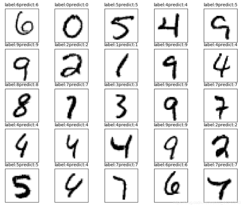
输出错误预测
#输出错误种类
def print_eer(labels,
              prediction):
    count=0;
    #找出错误预测
    compare_lists=(prediction==np.argmax(labels,1))
    #从len中,如果false,把i存入
    eer_lists=[i for i in range(len(compare_lists)) if compare_lists[i]==False]
    for x in eer_lists:
        print("index:",str(x),"标签值:",np.argmax(labels[x]),"预测值:",prediction[x])
        count=count+1
    print("预测错误总数:",len(eer_lists))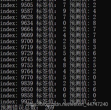
在损失函数交叉熵中log函数对log(0)不稳定,引起nan的存在


评论(0)
您还未登录,请登录后发表或查看评论