

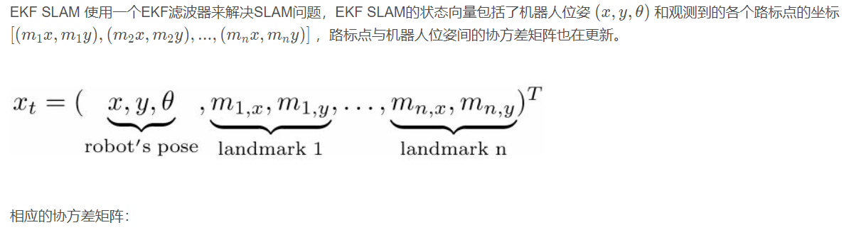
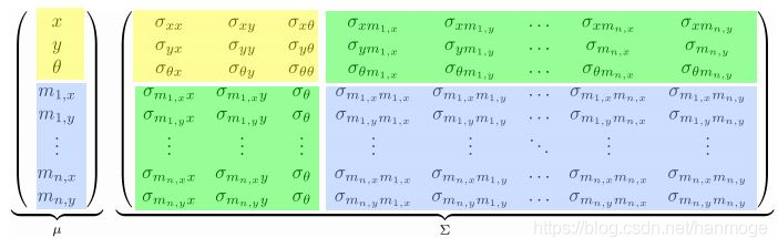
3 EKF SLAM
在上一节中我们看到的是扩展卡尔曼滤波在定位中的应用,EKF同样可以应用于SLAM问题中。在定位问题中,机器人接收到的观测值是其在二维空间中的x-y位置。如果机器人接收到的是跟周围环境有关的信息,例如机器人某时刻下距离某路标点的距离和角度,那么我们可以根据此时机器人自身位置的估计值,推测出该路标点在二维空间中的位置,将路标点的空间位置也作为待修正的状态量放入整个的状态向量中。
由此又引出了两个子问题:数据关联和状态扩增。
我们将通过以下python实例来理解ekf slam的原理(完整代码见原链接,有中文注释的附在了最后):
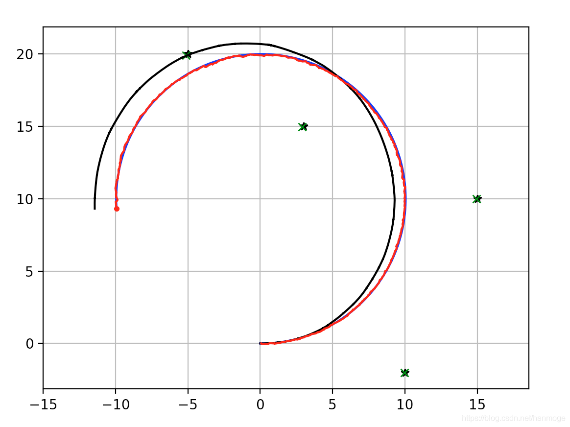
- 黑色星号: 路标点真实位置(代码中RFID数组代表真实位置)
- 绿色×: 路标点位置估计值
- 黑色线: 航迹推测方法得出的机器人轨迹
- 蓝色线: 轨迹真值
- 红色线: EKF SLAM得出的机器人轨迹
回想上一节的扩展卡尔曼滤波的公式:
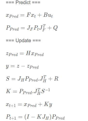
可以简写作:
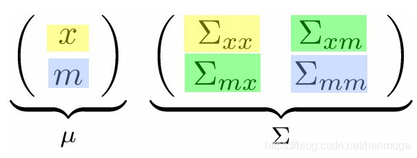
需要注意的是,由于状态向量中包含路标点位置坐标,所以随着机器人运动,观测到的路标点会越来越多,因此状态向量和状态协方差矩阵会不断变化。
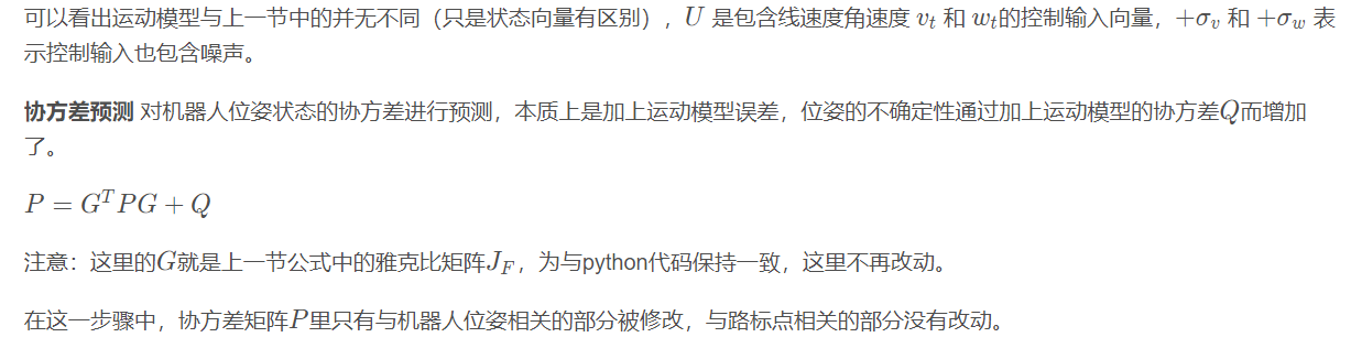
运动模型
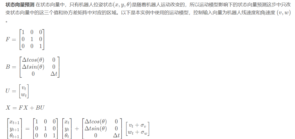
def motion_model(x, u):"""根据控制预测机器人位姿"""F = np.array([[1.0, 0, 0],[0, 1.0, 0],[0, 0, 1.0]])
B = np.array([[DT * math.cos(x[2, 0]), 0],[DT * math.sin(x[2, 0]), 0],[0.0, DT]])
x = (F @ x) + (B @ u)# 返回3x1return x
# 计算雅克比矩阵,与上一节相比并无不同,只不过因为机器人位姿状态向量少了一个元素,jF是3×3:def jacob_motion(x, u):Fx = np.hstack((np.eye(STATE_SIZE), np.zeros((STATE_SIZE, LM_SIZE * calc_n_lm(x)))))
jF = np.array([[0.0, 0.0, -DT * u[0] * math.sin(x[2, 0])],[0.0, 0.0, DT * u[0] * math.cos(x[2, 0])],[0.0, 0.0, 0.0]], dtype=np.float64)
G = np.eye(STATE_SIZE) + Fx.T @ jF @ Fx# 返回雅克比矩阵G(3x3),和对角矩阵Fx(实际上的np.eye(3))return G, Fx,
观测模型
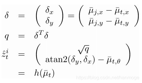
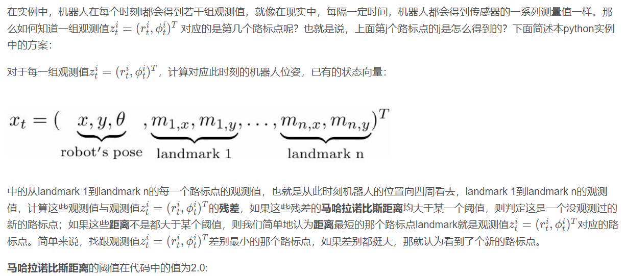
在这个实例中,观测模型比上一节要复杂,因为实例模拟的是激光雷达检测路标点获得的与机器人距离和角度的信息。观测值向量z zz包含的两个元素就是机器人与路标点的相对距离和角度,因此单个路标点在二维空间内的坐标就可以通过机器人在二维空间内的坐标得出: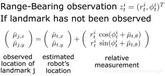
等式左边就是第j个路标点在二维空间内的坐标。
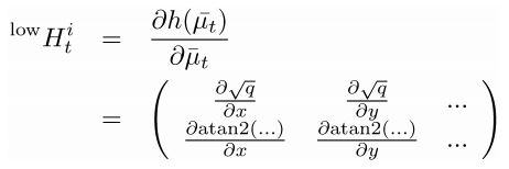
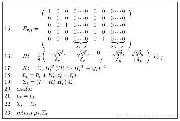
相应地,可以得到机器人位姿状态与单个路标点观测值之间的转换关系,也就是观测模型:
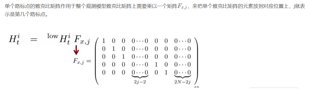
所以单个路标点的雅克比矩阵表示为:
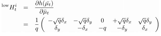

def calc_innovation(lm, xEst, PEst, z, LMid):"""Calculates the innovation based on expected position and landmark position:param lm: landmark position:param xEst: estimated position/state:param PEst: estimated covariance:param z: read measurements:param LMid: landmark id:returns: returns the innovation y, and the jacobian H, and S, used to calculate the Kalman Gain"""delta = lm - xEst[0:2]q = (delta.T @ delta)[0, 0]z_angle = math.atan2(delta[1, 0], delta[0, 0]) - xEst[2, 0]zp = np.array([[math.sqrt(q), pi_2_pi(z_angle)]]) # 对应以上的观测模型y = (z - zp).Ty[1] = pi_2_pi(y[1])# 放入delta的平方(标量),delta(2x1),状态向量和lm在状态向量中的序号+1H = jacob_h(q, delta, xEst, LMid + 1)S = H @ PEst @ H.T + R
return y, S, H
def jacob_h(q, delta, x, i):"""Calculates the jacobian of the measurement function:param q: the range from the system pose to the landmark:param delta: the difference between a landmark position and the estimated system position:param x: the state, including the estimated system position:param i: landmark id + 1:returns: the jacobian H"""sq = math.sqrt(q)G = np.array([[-sq * delta[0, 0], - sq * delta[1, 0], 0, sq * delta[0, 0], sq * delta[1, 0]],[delta[1, 0], - delta[0, 0], - q, - delta[1, 0], delta[0, 0]]]) # 单个路标点的雅克比矩阵G = G / q # 单个路标点的雅克比矩阵nLM = calc_n_lm(x) # 路标点总数F1 = np.hstack((np.eye(3), np.zeros((3, 2 * nLM))))
F2 = np.hstack((np.zeros((2, 3)), np.zeros((2, 2 * (i - 1))),np.eye(2), np.zeros((2, 2 * nLM - 2 * i))))F = np.vstack((F1, F2))H = G @ F
return H
其中jacob_h函数中的这几行代码:
F1 = np.hstack((np.eye(3), np.zeros((3, 2 * nLM))))F2 = np.hstack((np.zeros((2, 3)), np.zeros((2, 2 * (i - 1))),np.eye(2), np.zeros((2, 2 * nLM - 2 * i))))F = np.vstack((F1, F2))

import numpy as npnLM = 3 # 假设共有三个路标点i = 1F1 = np.hstack((np.eye(3), np.zeros((3, 2 * nLM))))F2 = np.hstack((np.zeros((2, 3)), np.zeros((2, 2 * (i - 1))),np.eye(2), np.zeros((2, 2 * nLM - 2 * i))))F = np.vstack((F1, F2))print(F1)print(F2)print(F)
[[ 1. 0. 0. 0. 0. 0. 0. 0. 0.][ 0. 1. 0. 0. 0. 0. 0. 0. 0.][ 0. 0. 1. 0. 0. 0. 0. 0. 0.]][[ 0. 0. 0. 1. 0. 0. 0. 0. 0.][ 0. 0. 0. 0. 1. 0. 0. 0. 0.]][[ 1. 0. 0. 0. 0. 0. 0. 0. 0.][ 0. 1. 0. 0. 0. 0. 0. 0. 0.][ 0. 0. 1. 0. 0. 0. 0. 0. 0.][ 0. 0. 0. 1. 0. 0. 0. 0. 0.][ 0. 0. 0. 0. 1. 0. 0. 0. 0.]]
i = 2F1 = np.hstack((np.eye(3), np.zeros((3, 2 * nLM))))F2 = np.hstack((np.zeros((2, 3)), np.zeros((2, 2 * (i - 1))),np.eye(2), np.zeros((2, 2 * nLM - 2 * i))))F = np.vstack((F1, F2))print(F1)print(F2)print(F)
[[ 1. 0. 0. 0. 0. 0. 0. 0. 0.][ 0. 1. 0. 0. 0. 0. 0. 0. 0.][ 0. 0. 1. 0. 0. 0. 0. 0. 0.]][[ 0. 0. 0. 0. 0. 1. 0. 0. 0.][ 0. 0. 0. 0. 0. 0. 1. 0. 0.]][[ 1. 0. 0. 0. 0. 0. 0. 0. 0.][ 0. 1. 0. 0. 0. 0. 0. 0. 0.][ 0. 0. 1. 0. 0. 0. 0. 0. 0.][ 0. 0. 0. 0. 0. 1. 0. 0. 0.][ 0. 0. 0. 0. 0. 0. 1. 0. 0.]]
i = 3F1 = np.hstack((np.eye(3), np.zeros((3, 2 * nLM))))F2 = np.hstack((np.zeros((2, 3)), np.zeros((2, 2 * (i - 1))),np.eye(2), np.zeros((2, 2 * nLM - 2 * i))))F = np.vstack((F1, F2))print(F1)print(F2)print(F)
[[ 1. 0. 0. 0. 0. 0. 0. 0. 0.][ 0. 1. 0. 0. 0. 0. 0. 0. 0.][ 0. 0. 1. 0. 0. 0. 0. 0. 0.]][[ 0. 0. 0. 0. 0. 0. 0. 1. 0.][ 0. 0. 0. 0. 0. 0. 0. 0. 1.]][[ 1. 0. 0. 0. 0. 0. 0. 0. 0.][ 0. 1. 0. 0. 0. 0. 0. 0. 0.][ 0. 0. 1. 0. 0. 0. 0. 0. 0.][ 0. 0. 0. 0. 0. 0. 0. 1. 0.][ 0. 0. 0. 0. 0. 0. 0. 0. 1.]]
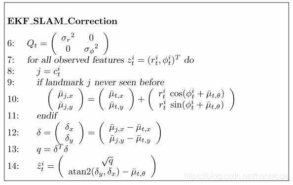
M_DIST_TH = 2.0 # Threshold of Mahalanobis distance for data association.## 注:马哈拉诺比斯距离Mahalanobis distance是由印度统计学家马哈拉诺比斯提出的,表示数据的协方差距离。## 它是一种有效的计算两个未知样本集的相似度的方法。与欧氏距离不同的是它考虑到各种特性之间的联系并且是尺度无关的,## 即独立于测量尺度(来自wiki)。
在实例中寻找匹配的路标点编号id的对应代码是:
def search_correspond_landmark_id(xAug, PAug, zi):"""Landmark association with Mahalanobis distance"""# 此时已有的LM的个数:nLM = calc_n_lm(xAug)
min_dist = []
for i in range(nLM):# 返回第i个已有LM的坐标lm:lm = get_landmark_position_from_state(xAug, i)# 放入第i个已有LM的坐标lm、机器人位姿预测过的状态向量xAug和variance PAug、待比较的新观测ziy, S, H = calc_innovation(lm, xAug, PAug, zi, i)# 由残差y计算Mahalanobis distance:y.T @ np.linalg.inv(S) @ ymin_dist.append(y.T @ np.linalg.inv(S) @ y)
min_dist.append(M_DIST_TH) # new landmark
min_id = min_dist.index(min(min_dist))
return min_id
这种根据残差的马哈拉诺比斯距离最小来寻找匹配的路标点只是一种理想化的简单处理方式,实际应用中的“data association”会复杂得多。

# Extend state and covariance matrix
xAug = np.vstack((xEst, calc_landmark_position(xEst, z[iz, :])))
PAug = np.vstack((np.hstack((PEst, np.zeros((len(xEst), LM_SIZE)))),
np.hstack((np.zeros((LM_SIZE, len(xEst))), initP))))
xEst = xAug
PEst = PAug

最后再说一点此实例中有关仿真数据生成的内容,在observation函数中,根据机器人位姿真值决定机器人可以看到哪几个路标点,再将这几个路标点的观测值人为加上噪声。
参考链接:
SLAM笔记五——EKF-SLAM
PythonRobotics/SLAM/EKFSLAM
附上带中文注释的完整代码:
"""Extended Kalman Filter SLAM example
author: Atsushi Sakai (@Atsushi_twi)
https://github.com/AtsushiSakai/PythonRobotics/tree/master/SLAM/EKFSLAM"""
import math
import matplotlib.pyplot as pltimport numpy as np
# 在这里我对代码做了一些改动,原代码的Cx不太便于读者理解:# EKF state covariance: 3x3 sizeQ = np.diag([0.5, 0.5, np.deg2rad(30.0)]) ** 2# landmark observation covariance: 2x2 sizeR = np.diag([0.5, 0.5])**2
# Simulation parameterQ_sim = np.diag([0.2, np.deg2rad(1.0)]) ** 2R_sim = np.diag([1.0, np.deg2rad(10.0)]) ** 2
DT = 0.1 # time tick [s]SIM_TIME = 50.0 # simulation time [s]MAX_RANGE = 20.0 # maximum observation rangeM_DIST_TH = 2.0 # Threshold of Mahalanobis distance for data association.## 注:马哈拉诺比斯距离是由印度统计学家马哈拉诺比斯提出的,表示数据的协方差距离。它是一种有效的计算两个未知样本集的相似度的方法。与欧氏距离不同的是它考虑到各种特性之间的联系并且是尺度无关的,即独立于测量尺度(来自wiki)。STATE_SIZE = 3 # State size [x,y,yaw]LM_SIZE = 2 # LM state size [x,y]
show_animation = True
def ekf_slam(xEst, PEst, u, z):# Predict# 预测过程只与运动模型有关S = STATE_SIZE# 返回运动模型雅克比G和对角矩阵FxG, Fx = jacob_motion(xEst[0:S], u)# 返回机器人位姿的在含噪控制下的预测:xEst[0:S] = motion_model(xEst[0:S], u)# 更新机器人位姿的PPEst[0:S, 0:S] = G.T @ PEst[0:S, 0:S] @ G + Fx.T @ Q @ Fx# 给Landmark准备的varianceinitP = np.eye(2)
# Update# 对在此时刻新得到的一组z含噪观测,对z中的每一个元素做操作:for iz in range(len(z[:, 0])): # for each observationmin_id = search_correspond_landmark_id(xEst, PEst, z[iz, 0:2])
nLM = calc_n_lm(xEst)# 在函数search_correspond_landmark_id中,把M_DIST_TH放在了最后一个,# 又因为已有的LM的序号值范围是(0至(nLM-1)),所以最后一个值M_DIST_TH的序号就是nLM,# 所以如果min_id等于nLM,意味着新观测z[iz, 0:2]与所有已有观测的马哈拉诺比斯距离都超过了M_DIST_TH,# 即这是一个以前没看到过的LM:if min_id == nLM:print("New LM")# Extend state and covariance matrixxAug = np.vstack((xEst, calc_landmark_position(xEst, z[iz, :])))PAug = np.vstack((np.hstack((PEst, np.zeros((len(xEst), LM_SIZE)))),np.hstack((np.zeros((LM_SIZE, len(xEst))), initP))))xEst = xAugPEst = PAug# 如果min_id不等于nLM,则认为这是一个已经观测过的LM,# 马哈拉诺比斯距离最小的那个,也就是min_id指向的那个就是对应的已观测LM:lm = get_landmark_position_from_state(xEst, min_id)y, S, H = calc_innovation(lm, xEst, PEst, z[iz, 0:2], min_id)
K = (PEst @ H.T) @ np.linalg.inv(S)xEst = xEst + (K @ y)PEst = (np.eye(len(xEst)) - (K @ H)) @ PEst
xEst[2] = pi_2_pi(xEst[2])
return xEst, PEst
def calc_input():v = 1.0 # [m/s]yaw_rate = 0.1 # [rad/s]u = np.array([[v, yaw_rate]]).Treturn u
def observation(xTrue, xd, u, RFID):"""仿真过程"""xTrue = motion_model(xTrue, u)
z = np.zeros((0, 3))
for i in range(len(RFID[:, 0])):
dx = RFID[i, 0] - xTrue[0, 0]dy = RFID[i, 1] - xTrue[1, 0]# 计算机器人位姿真值与路标点的距离dd = math.hypot(dx, dy)angle = pi_2_pi(math.atan2(dy, dx) - xTrue[2, 0])# 如果距离d小于阈值,代表机器人可以看到这个路标点:if d <= MAX_RANGE:dn = d + np.random.randn() * Q_sim[0, 0] ** 0.5 # add noiseangle_n = angle + np.random.randn() * Q_sim[1, 1] ** 0.5 # add noisezi = np.array([dn, angle_n, i])z = np.vstack((z, zi))
# add noise to inputud = np.array([[u[0, 0] + np.random.randn() * R_sim[0, 0] ** 0.5,u[1, 0] + np.random.randn() * R_sim[1, 1] ** 0.5]]).T
xd = motion_model(xd, ud)# 返回xTrue(3x1), z含噪观测(3xnLM含RFID的id),xd(3x1),ud含噪控制(2x1)return xTrue, z, xd, ud
def motion_model(x, u):"""根据控制预测机器人位姿"""F = np.array([[1.0, 0, 0],[0, 1.0, 0],[0, 0, 1.0]])
B = np.array([[DT * math.cos(x[2, 0]), 0],[DT * math.sin(x[2, 0]), 0],[0.0, DT]])
x = (F @ x) + (B @ u)# 返回3x1return x
def calc_n_lm(x):"""返回Landmark的个数"""n = int((len(x) - STATE_SIZE) / LM_SIZE)return n
def jacob_motion(x, u):Fx = np.hstack((np.eye(STATE_SIZE), np.zeros((STATE_SIZE, LM_SIZE * calc_n_lm(x)))))
jF = np.array([[0.0, 0.0, -DT * u[0] * math.sin(x[2, 0])],[0.0, 0.0, DT * u[0] * math.cos(x[2, 0])],[0.0, 0.0, 0.0]], dtype=np.float64)
G = np.eye(STATE_SIZE) + Fx.T @ jF @ Fx# 返回雅克比矩阵G(3x3),和对角矩阵Fx(实际上的np.eye(3))return G, Fx,
def calc_landmark_position(x, z):"""根据观测z和预测后的x状态向量,计算LM的坐标位置"""zp = np.zeros((2, 1))
zp[0, 0] = x[0, 0] + z[0] * math.cos(x[2, 0] + z[1])zp[1, 0] = x[1, 0] + z[0] * math.sin(x[2, 0] + z[1])
return zp
def get_landmark_position_from_state(x, ind):"""根据lm在状态向量中的id查找lm的坐标:"""lm = x[STATE_SIZE + LM_SIZE * ind: STATE_SIZE + LM_SIZE * (ind + 1), :]
return lm
def search_correspond_landmark_id(xAug, PAug, zi):"""Landmark association with Mahalanobis distance"""# 此时已有的LM的个数:nLM = calc_n_lm(xAug)
min_dist = []
for i in range(nLM):# 返回第i个已有LM的坐标lm:lm = get_landmark_position_from_state(xAug, i)# 放入第i个已有LM的坐标lm、机器人位姿预测过的状态向量xAug和variance PAug、待比较的新观测ziy, S, H = calc_innovation(lm, xAug, PAug, zi, i)# 由残差y计算Mahalanobis distance:y.T @ np.linalg.inv(S) @ ymin_dist.append(y.T @ np.linalg.inv(S) @ y)
min_dist.append(M_DIST_TH) # new landmark
min_id = min_dist.index(min(min_dist))
return min_id
def calc_innovation(lm, xEst, PEst, z, LMid):"""Calculates the innovation based on expected position and landmark position:param lm: landmark position:param xEst: estimated position/state:param PEst: estimated covariance:param z: read measurements:param LMid: landmark id:returns: returns the innovation y, and the jacobian H, and S, used to calculate the Kalman Gain"""delta = lm - xEst[0:2]q = (delta.T @ delta)[0, 0]z_angle = math.atan2(delta[1, 0], delta[0, 0]) - xEst[2, 0]zp = np.array([[math.sqrt(q), pi_2_pi(z_angle)]])y = (z - zp).Ty[1] = pi_2_pi(y[1])# 放入delta的平方(标量),delta(2x1),状态向量和lm在状态向量中的序号+1H = jacob_h(q, delta, xEst, LMid + 1)S = H @ PEst @ H.T + R
return y, S, H
def jacob_h(q, delta, x, i):"""Calculates the jacobian of the measurement function:param q: the range from the system pose to the landmark:param delta: the difference between a landmark position and the estimated system position:param x: the state, including the estimated system position:param i: landmark id + 1:returns: the jacobian H"""sq = math.sqrt(q)G = np.array([[-sq * delta[0, 0], - sq * delta[1, 0], 0, sq * delta[0, 0], sq * delta[1, 0]],[delta[1, 0], - delta[0, 0], - q, - delta[1, 0], delta[0, 0]]])G = G / qnLM = calc_n_lm(x)F1 = np.hstack((np.eye(3), np.zeros((3, 2 * nLM))))
F2 = np.hstack((np.zeros((2, 3)), np.zeros((2, 2 * (i - 1))),np.eye(2), np.zeros((2, 2 * nLM - 2 * i))))F = np.vstack((F1, F2))H = G @ F
return H
def pi_2_pi(angle):"""将角度范围限定在[-pi,pi]"""return (angle + math.pi) % (2 * math.pi) - math.pi
def main():print(__file__ + " start!!")
time = 0.0
# RFID positions [x, y]RFID = np.array([[10.0, -2.0],[15.0, 10.0],[3.0, 15.0],[-5.0, 20.0]])
# State Vector [x y yaw]'xEst = np.zeros((STATE_SIZE, 1))xTrue = np.zeros((STATE_SIZE, 1))PEst = np.eye(STATE_SIZE)
xDR = np.zeros((STATE_SIZE, 1)) # Dead reckoning
# historyhxEst = xEsthxTrue = xTruehxDR = xTrue
while SIM_TIME >= time:time += DTu = calc_input() #真值
xTrue, z, xDR, ud = observation(xTrue, xDR, u, RFID)# 返回xTrue(3x1), z含噪观测(3xnLM含RFID的id),xDR(3x1),ud含噪控制(2x1)
xEst, PEst = ekf_slam(xEst, PEst, ud, z)
x_state = xEst[0:STATE_SIZE]
# store data historyhxEst = np.hstack((hxEst, x_state))hxDR = np.hstack((hxDR, xDR))hxTrue = np.hstack((hxTrue, xTrue))
if show_animation: # pragma: no coverplt.cla()# for stopping simulation with the esc key.plt.gcf().canvas.mpl_connect('key_release_event',lambda event: [exit(0) if event.key == 'escape' else None])
plt.plot(RFID[:, 0], RFID[:, 1], "*k")plt.plot(xEst[0], xEst[1], ".r")
# plot landmarkfor i in range(calc_n_lm(xEst)):plt.plot(xEst[STATE_SIZE + i * 2],xEst[STATE_SIZE + i * 2 + 1], "xg")
plt.plot(hxTrue[0, :],hxTrue[1, :], "-b")plt.plot(hxDR[0, :],hxDR[1, :], "-k")plt.plot(hxEst[0, :],hxEst[1, :], "-r")plt.axis("equal")plt.grid(True)plt.pause(0.001)
if __name__ == '__main__':main()


评论(0)
您还未登录,请登录后发表或查看评论