快速入门keras CNN 小花分类程序

微欧小v

分类：机器学习

发布时间 2022.09.27阅读数 2386 评论数 0

1 收集下载数据

2 读取本地数据

3 搭建网络模型CNN

4 编写训练文件 train.py

5 编写预测推理文件predict.py

本程序使用tensorflow的keras 库，适用tf版本为2.9。

导入常用的库

# -*- coding:utf-8 -*-
import matplotlib.pyplot as plt
import numpy as np
# TensorFlow and tf.keras
import tensorflow as tf
from tensorflow import keras

# Helper libraries
import numpy as np
# import matplotlib.pyplot as plt
import tensorflow as tf

from tensorflow import keras
from tensorflow.keras import layers
from tensorflow.keras.models import Sequential
print(tf.__version__)
import os
#import PIL
import  pathlib

下载小花库链接：https://pan.baidu.com/s/1-SK-mcS6MNXoa0i60g7FEw

提取码：dmi7

flower_photos的文件夹内部

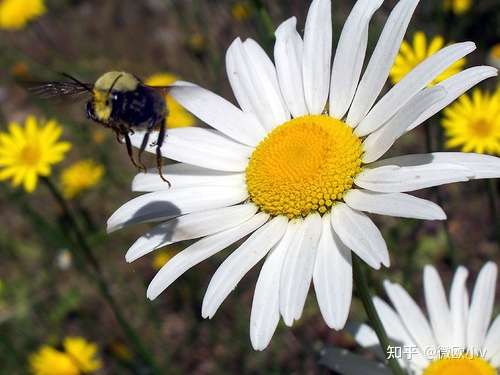
读取文件夹中的花，兵将花分成8：2训练集和验证集。

data_dir = pathlib.Path('E:/lide/keras/flower_photos')
print(data_dir)
image_count = len(list(data_dir.glob('*/*.jpg')))
print(image_count)

batch_size = 32
img_height = 180
img_width = 180
#use 8:2 train and valigation
train_ds = tf.keras.utils.image_dataset_from_directory(
  data_dir,
  validation_split=0.2,
  subset="training",
  seed=123,
  image_size=(img_height, img_width),
  batch_size=batch_size)
#验证集
val_ds = tf.keras.utils.image_dataset_from_directory(
  data_dir,
  validation_split=0.2,
  subset="validation",
  seed=123,
  image_size=(img_height, img_width),
  batch_size=batch_size)

#class_names = train_ds.class_names
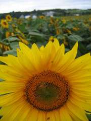
class_names = ['1.daisy', '2.dandelion', '3.roses', '4.sunflowers', '5.tulips']
print(class_names)

上段执行后的结果为

3640
Found 3640 files belonging to 5 classes.
Using 2912 files for training.

可见有3640个样本，其中2912个样本将作为训练样本。

训练文件 train.py

# -*- coding:utf-8 -*-
import matplotlib.pyplot as plt
import numpy as np
# TensorFlow and tf.keras
import tensorflow as tf
from tensorflow import keras

# Helper libraries
import numpy as np
# import matplotlib.pyplot as plt
import tensorflow as tf

from tensorflow import keras
from tensorflow.keras import layers
from tensorflow.keras.models import Sequential
print(tf.__version__)
import os
#import PIL
import  pathlib


data_dir = pathlib.Path('E:/lide/keras/flower_photos')
print(data_dir)
image_count = len(list(data_dir.glob('*/*.jpg')))
print(image_count)

batch_size = 32
img_height = 180
img_width = 180
#use 8:2 train and valigation
train_ds = tf.keras.utils.image_dataset_from_directory(
  data_dir,
  validation_split=0.2,
  subset="training",
  seed=123,
  image_size=(img_height, img_width),
  batch_size=batch_size)
#验证集
val_ds = tf.keras.utils.image_dataset_from_directory(
  data_dir,
  validation_split=0.2,
  subset="validation",
  seed=123,
  image_size=(img_height, img_width),
  batch_size=batch_size)

#class_names = train_ds.class_names
class_names = ['1.daisy', '2.dandelion', '3.roses', '4.sunflowers', '5.tulips']
print(class_names)

for image_batch, labels_batch in train_ds:
  print(image_batch.shape)
  print(labels_batch.shape)
  break

AUTOTUNE = tf.data.AUTOTUNE

train_ds = train_ds.cache().shuffle(1000).prefetch(buffer_size=AUTOTUNE)
val_ds = val_ds.cache().prefetch(buffer_size=AUTOTUNE)

normalization_layer = layers.Rescaling(1./255)
normalized_ds = train_ds.map(lambda x, y: (normalization_layer(x), y))
image_batch, labels_batch = next(iter(normalized_ds))
first_image = image_batch[0]
# Notice the pixel values are now in `[0,1]`.
print(np.min(first_image), np.max(first_image))

num_classes = len(class_names)

model = Sequential([
  layers.Rescaling(1./255, input_shape=(img_height, img_width, 3)),
  layers.Conv2D(16, 3, padding='same', activation='relu'),
  layers.MaxPooling2D(),
  layers.Conv2D(32, 3, padding='same', activation='relu'),
  layers.MaxPooling2D(),
  layers.Conv2D(64, 3, padding='same', activation='relu'),
  layers.MaxPooling2D(),
  layers.Dropout(0.2),
  layers.Flatten(),
  layers.Dense(128, activation='relu'),
  layers.Dense(num_classes)
])

model.compile(optimizer='adam',
              loss=tf.keras.losses.SparseCategoricalCrossentropy(from_logits=True),
              metrics=['accuracy'])
model.summary()

epochs=10
history = model.fit(
  train_ds,
  validation_data=val_ds,
  epochs=epochs
)
model.save("finalmodel.h5")
#可视化
acc = history.history['accuracy']
val_acc = history.history['val_accuracy']

loss = history.history['loss']
val_loss = history.history['val_loss']

epochs_range = range(epochs)

plt.figure(figsize=(8, 8))
plt.subplot(1, 2, 1)
plt.plot(epochs_range, acc, label='Training Accuracy')
plt.plot(epochs_range, val_acc, label='Validation Accuracy')
plt.legend(loc='lower right')
plt.title('Training and Validation Accuracy')

plt.subplot(1, 2, 2)
plt.plot(epochs_range, loss, label='Training Loss')
plt.plot(epochs_range, val_loss, label='Validation Loss')
plt.legend(loc='upper right')
plt.title('Training and Validation Loss')
plt.show()

开始训练

Found 3640 files belonging to 5 classes.
Using 728 files for validation.
['1.daisy', '2.dandelion', '3.roses', '4.sunflowers', '5.tulips']
(32, 180, 180, 3)
(32,)
0.0 0.9988043
Model: "sequential"
_________________________________________________________________
 Layer (type)                Output Shape              Param #
=================================================================
 rescaling_1 (Rescaling)     (None, 180, 180, 3)       0

 conv2d (Conv2D)             (None, 180, 180, 16)      448

 max_pooling2d (MaxPooling2D  (None, 90, 90, 16)       0
 )

 conv2d_1 (Conv2D)           (None, 90, 90, 32)        4640

 max_pooling2d_1 (MaxPooling  (None, 45, 45, 32)       0
 2D)

 conv2d_2 (Conv2D)           (None, 45, 45, 64)        18496

 max_pooling2d_2 (MaxPooling  (None, 22, 22, 64)       0
 2D)

 dropout (Dropout)           (None, 22, 22, 64)        0

 flatten (Flatten)           (None, 30976)             0

 dense (Dense)               (None, 128)               3965056

 dense_1 (Dense)             (None, 5)                 645

=================================================================
Total params: 3,989,285
Trainable params: 3,989,285
91/91 [==============================] - 23s 255ms/step - loss: 0.1849 - accuracy: 0.9406 - val_loss: 1.3267 - val_accuracy: 0.6621
Epoch 8/10
91/91 [==============================] - 23s 253ms/step - loss: 0.0950 - accuracy: 0.9763 - val_loss: 1.7882 - val_accuracy: 0.6621
Epoch 9/10
91/91 [==============================] - 23s 255ms/step - loss: 0.0730 - accuracy: 0.9794 - val_loss: 1.7537 - val_accuracy: 0.6621
Epoch 10/10
91/91 [==============================] - 23s 253ms/step - loss: 0.0498 - accuracy: 0.9863 - val_loss: 1.5840 - val_accuracy: 0.6580

训练完成。发现该网络有11层，共计3989285个参数，迭代训练10次，每次91步（样本数*训练比/batch_size,这里就是3640*0.8/32 =91），

Image classification | TensorFlow Core

下图中验证集的准确率持续在0.6-0.7之间波动，而训练集的准确率在持续升高。

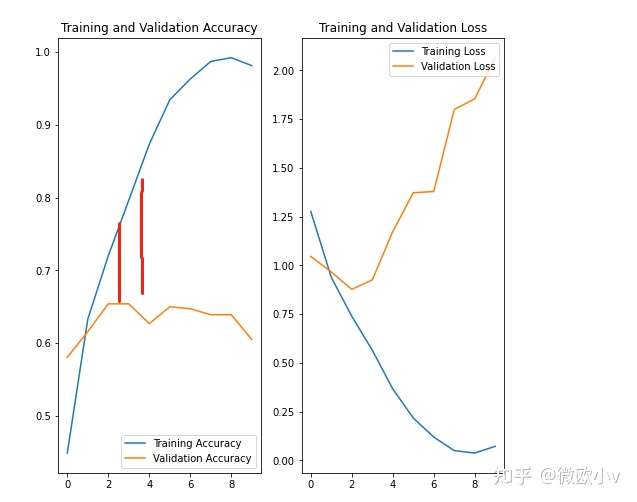
发生过拟合。过拟合是指未见过的准确率不如在训练数据上的表现得分高。过拟合的模型会“记住”训练数据集中的噪声和细节，将这些糟糕的情况放大，从而对模型在新数据上的表现产生负面影响。

过拟合的解决策略

Overfit and underfit | TensorFlow Core

这是很典型的过度拟合问题。

解决方案：

1 增加样本多样化和样本训练数量即数据增强。

2另一种减少过拟合的技术是在网络中引入dropout正则化。它会在训练过程中从层中随机丢弃一些输出单元，以减小过度重合的机会。

model = Sequential([
  data_augmentation,
  layers.Rescaling(1./255),
  layers.Conv2D(16, 3, padding='same', activation='relu'),
  layers.MaxPooling2D(),
  layers.Conv2D(32, 3, padding='same', activation='relu'),
  layers.MaxPooling2D(),
  layers.Conv2D(64, 3, padding='same', activation='relu'),
  layers.MaxPooling2D(),
  layers.Dropout(0.2), #丢掉20%的输出单元
  layers.Flatten(),
  layers.Dense(128, activation='relu'),
  layers.Dense(num_classes)
])

并保存为 finalmodel.h5 。

在predict.py 内部加载模型并随便调用一张dande的图片推理。

# -*- coding:utf-8 -*-
import matplotlib.pyplot as plt
import numpy as np
# TensorFlow and tf.keras
import tensorflow as tf
from tensorflow import keras

# Helper libraries
import numpy as np
# import matplotlib.pyplot as plt
import tensorflow as tf

from tensorflow import keras
from tensorflow.keras import layers
from tensorflow.keras.models import Sequential
print(tf.__version__)
import os
#import PIL
import  pathlib
from keras.models import load_model
 


#roses = list(data_dir.glob('3.roses/*'))
#PIL.Image.open(str(roses[0]))
batch_size = 32
img_height = 180
img_width = 180
 
sunflower_path = 'E:/lide/keras/test/dande.jpg'

img = tf.keras.utils.load_img(
    sunflower_path, target_size=(img_height, img_width)
)
img_array = tf.keras.utils.img_to_array(img)
img_array = tf.expand_dims(img_array, 0) # Create a batch
model = load_model('finalmodel.h5')
 
predictions = model.predict(img_array)
score = tf.nn.softmax(predictions[0])
class_names = ['1.daisy', '2.dandelion', '3.roses', '4.sunflowers', '5.tulips']
print(
    "This image most likely belongs to {} with a {:.2f} percent confidence."
    .format(class_names[np.argmax(score)], 100 * np.max(score))
)

python predict.py 推理结果为

1/1 [==============================] - 0s 111ms/step
This image most likely belongs to 2.dandelion with a 49.54 percent confidence.
(tf) PS E:\lide\keras>

机器学习深度学习神经网络 Keras CNN

转载原出处：https://zhuanlan.zhihu.com/p/551792561

打赏 0

上一篇：开源的地图路径规划网站

快速入门keras CNN 小花分类程序

微欧小v

为你推荐

精选经典文献阅读之--EdgeYOLO(边缘设备YOLO目标检测)

Pytorch 3. 创建一个神经网络

使用keras全连接网络训练mnist手写数字识别并输出可视化训练过程以及预测结果

【机器学习】【笔记】sklearn中的核函数

强化学习在游戏AI中的应用与挑战

深度残差收缩网络

关于作者

微欧小v

5

0

0

2

matterport MASKRCNN识别水坑

开源的地图路径规划网站

matterport MASKRCNN识别道路井盖

相关推荐

机器学习——Python实现KNN识别MNIST手写数字体

决策树枝干的拓展

精选Intel深度摄像头RealSense D435（实感双目摄像头）和目标检测结合使用

改进YOLOv8系列：即插即用新的注意力机制RFAConv

NLP学习之使用pytorch搭建textCNN模型进行中文文本分类

Tensorflow,Keras环境下实现EfficientNet实例

热门泡泡

30积分失眠，聊聊自己搞ROS的心得体会吧

ros学习路线

30积分 TF_REPEATED_DATA ignoring data错误

各位大佬，有什么ROS定位算法推荐吗

5积分想买能用ROS2的开发套件。或者开发板

5积分 ros中启动gazebo时报错

给作者打赏

快速入门keras CNN 小花分类程序

微欧小v

为你推荐

精选经典文献阅读之--EdgeYOLO(边缘设备YOLO目标检测)

Pytorch 3. 创建一个神经网络

使用keras全连接网络训练mnist手写数字识别并输出可视化训练过程以及预测结果

【机器学习】【笔记】sklearn中的核函数

强化学习在游戏AI中的应用与挑战

深度残差收缩网络

评论（0）

关于作者

微欧小v

5

0

0

2

matterport MASKRCNN识别水坑

开源的地图路径规划网站

matterport MASKRCNN识别道路井盖

相关推荐

机器学习——Python实现KNN识别MNIST手写数字体

决策树枝干的拓展

精选Intel深度摄像头RealSense D435（实感双目摄像头）和目标检测结合使用

改进YOLOv8系列：即插即用新的注意力机制RFAConv

NLP学习之使用pytorch搭建textCNN模型进行中文文本分类

Tensorflow,Keras环境下实现EfficientNet实例

热门泡泡

30积分 失眠，聊聊自己搞ROS的心得体会吧

ros学习路线

30积分 TF_REPEATED_DATA ignoring data错误

各位大佬，有什么ROS定位算法推荐吗

5积分 想买能用ROS2的开发套件。或者开发板

5积分 ros中启动gazebo时报错

给作者打赏

忘记密码

修改头像

添加你感兴趣的标签

举报类型（必选）

举报详情（选填）

30积分失眠，聊聊自己搞ROS的心得体会吧

5积分想买能用ROS2的开发套件。或者开发板