

趁着时间多,今天继续学习tensorflow的知识,以前只知道复现搭建配环境,没从基础只是开始,所以从基础知识开始学习,收获了很多,对深度学习的理解有了更加深入的认识。
深度神经网络已经不能满足我了,今天是卷积神经网络的搭建与训练CIFA10,其实步骤都是一样的。

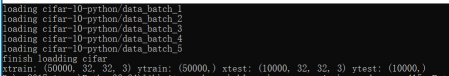
数据获取
#读一个批次
def load_cifar_batch(filename):
    with open(filename,'rb') as f:
        data_dict=p.load(f,encoding='bytes')
        images =data_dict[b'data']
        labels=data_dict[b'labels']
        images=images.reshape(10000,3,32,32)
        images=images.transpose(0,2,3,1)
        labels=np.array(labels)
        return images,labels
#读所有样本,总共5批训练,一个测试
def load_cifar_data(data_dir):
    images_train=[]
    labels_train=[]
    for i in range(5):
        f=os.path.join(data_dir,'data_batch_%d'%(i+1))
        print('loading',f)
        image_batch,label_batch=load_cifar_batch(f)
        images_train.append(image_batch)
        labels_train.append(label_batch)
        xtrain=np.concatenate(images_train)
        ytrain=np.concatenate(labels_train)
        del label_batch,image_batch
    xtest,ytest=load_cifar_batch(os.path.join(data_dir,'test_batch'))
    print('finish loadding cifar')
    return xtrain,ytrain,xtest,ytest
#读取数据
data_dir='cifar-10-python/'
xtrain,ytrain,xtest,ytest=load_cifar_data(data_dir)
print('xtrain:',xtrain.shape,'ytrain:',ytrain.shape,'xtest:',xtest.shape,'ytest:',ytest.shape)
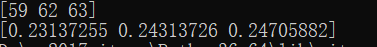
数据预处理
#数据预处理
#归一化
#print(xtrain[0][0][0])
xtrain_normalize=xtrain.astype('float32')/255.0
xtest_normalize=xtest.astype('float32')/255.0
#print(xtrain_normalize[0][0][0])
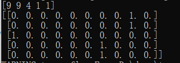
#标签进行预处理,转换成独热编码
from sklearn.preprocessing import OneHotEncoder
encoder=OneHotEncoder(sparse=False)
yy=[[0],[1],[2],[3],[4],[5],[6],[7],[8],[9]]
encoder.fit(yy)
ytrain_reshape=ytrain.reshape(-1,1)
ytrain_onehot=encoder.transform(ytrain_reshape)
ytest_reshape=ytest.reshape(-1,1)
ytest_onehot=encoder.transform(ytest_reshape)
#print(ytrain[1:6])
#print(ytest_onehot[1:6])
展示x归一化
展示y独热
模型构建
#构建卷积神经网络
#1输入2卷积2降采样1全连接1输出
tf.reset_default_graph()
#定义共享函数
#权值
def weight(shape):
    return tf.Variable(tf.truncated_normal(shape,stddev=0.1),name='w')
#偏置
def bias(shape):
    return tf.Variable(tf.constant(0.1,shape=shape),name='b')
#定义卷积操作
#定义步长
def conv2d(x,w):
    return tf.nn.conv2d(x,w,strides=[1,1,1,1],padding='SAME')
#定义池化
def max_pool_2(x):
    return tf.nn.max_pool(x,ksize=[1,2,2,1],strides=[1,2,2,1],padding='SAME')
#定义网络结构
#输入层32*32*3通
with tf.name_scope('input_layer'):
    x=tf.placeholder('float',shape=[None,32,32,3],name='x')
#第一层卷积
with tf.name_scope('conv1'):
    w1=weight([3,3,3,32])#卷积核宽、高、输入通、输出通
    b1=bias([32])#输出通
    conv_1=conv2d(x,w1)+b1#卷积加偏置
    conv_1=tf.nn.relu(conv_1)#激活
#第一层池化,最大池化
with tf.name_scope('pool1'):
    pool_1=max_pool_2(conv_1)
#第二层卷积
with tf.name_scope('conv2'):
    w2=weight([3,3,32,64])
    b2=bias([64])
    conv_2=conv2d(pool_1,w2)+b2
    conv_2=tf.nn.relu(conv_2)
#第二层池化,最大池化
with tf.name_scope('pool2'):
    pool_2=max_pool_2(conv_2)
#全连接层,4096=64*8*8,第二层池化得出,
with tf.name_scope('fc'):
    w3=weight([4096,128])#128神经元
    b3=bias([128])
    flat=tf.reshape(pool_2,[-1,4096])
    h=tf.nn.relu(tf.matmul(flat,w3)+b3)#叉乘连接
    h_dropout=tf.nn.dropout(h,keep_prob=0.8)#避免过拟合
#输出层,输出十个类别
with tf.name_scope('out_layer'):
    w4=weight([128,10])
    b4=bias([10])
    pred=tf.nn.softmax(tf.matmul(h_dropout,w4)+b4)
优化器损失及超参
#构建模型
with tf.name_scope('optimizer'):
    #占位符
    y=tf.placeholder('float',shape=[None,10],name='y')
    #损失函数
    loss_function=tf.reduce_mean(tf.nn.softmax_cross_entropy_with_logits(logits=pred,labels=y))
    #优化器
    optimizer=tf.train.AdamOptimizer(learning_rate=0.0001).minimize(loss_function)
#定义准确率
with tf.name_scope('evaluation'):
    correct_prediction=tf.equal(tf.argmax(pred,1),tf.argmax(y,1))
    accuracy=tf.reduce_mean(tf.cast(correct_prediction,'float'))
#设置超参
train_epochs=30
batch_size=50
total_batch=int(len(xtrain)/batch_size)
epoch_list=[];accuracy_list=[];loss_list=[];
epoch=tf.Variable(0,name='epoch',trainable=False)
#记录时间并初始化
start_time=time()
sess=tf.Session()
sess.run(tf.global_variables_initializer())
训练模型
#迭代训练
#获取数据
def get_train(number,batch_size):
    return xtrain_normalize[number*batch_size:(number+1)*batch_size],ytrain_onehot[number*batch_size:(number+1)*batch_size]
#训练
for ep in range(start,train_epochs):
    for i in range(total_batch):
        batch_x,batch_y=get_train(i,batch_size)
        sess.run(optimizer,feed_dict={x:batch_x,y:batch_y})
        if i%100==0:
            print('step{}:'.format(i),'finished')
    loss,acc=sess.run([loss_function,accuracy],feed_dict={x:batch_x,y:batch_y})
    epoch_list.append(ep+1)
    loss_list.append(loss)
    accuracy_list.append(acc)
    print('train epoch:',ep+1,'loss:','{:6f}'.format(loss),'accuracy:',acc)
    #保存
    saver.save(sess,os.path.join(ckpt_dir,'cifar10_cnn{:6d}.ckpt'.format(ep+1)))
    print('已保存:',ep+1)
    sess.run(epoch.assign(ep+1))
模型保存及载入
#设置断点断训
#判断是否有文件
ckpt_dir='cifa10_log'
if not os.path.exists(ckpt_dir):
    os.makedirs(ckpt_dir)
#保存加载参数,准备继续训练
saver=tf.train.Saver(max_to_keep=1)
ckpt=tf.train.latest_checkpoint(ckpt_dir)
if ckpt!=None:
    saver.restore(sess,ckpt)
else:
    print('New_training')
start=sess.run(epoch)
print('epoch{}:'.format(start+1))
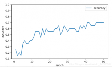
结果可视化
total_time=time()-start_time
print('训练结束,总用时:',total_time)
plt.plot(epoch_list,accuracy_list,label='accuracy')
fig=plt.gcf()
fig.set_size_inches(4,2)
plt.ylim(0.1,1)
plt.ylabel('accuracy')
plt.xlabel('epoch')
plt.legend()
plt.show()
plt.plot(epoch_list,loss_list,label='loss')
fig=plt.gcf()
fig.set_size_inches(4,2)
plt.ylim(0.1,1)
plt.ylabel('loss')
plt.xlabel('epoch')
plt.legend()
plt.show()
test_total_batch=int(len(xtest_normalize)/batch_size)
test_acc_sum=0.0
for i in range(test_total_batch):
test_image_batch=xtest_normalize[i*batch_size:(i+1)*batch_size]
test_label_batch=ytest_onehot[i*batch_size:(i+1)*batch_size]
tess_batch_acc=sess.run(accuracy,feed_dict={x:test_image_batch,y:test_label_batch})
test_acc_sum+=tess_batch_acc
test_acc=float(test_acc_sum/test_total_batch)
print('test_accuracy{:.6f}'.format(test_acc))
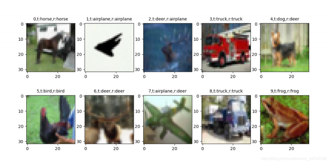
test_pred=sess.run(pred,feed_dict={x:xtest_normalize[:30]})
prediction_result=sess.run(tf.argmax(test_pred,1))
plot_images_label(xtest,ytest,prediction_result,20,10)


评论(0)
您还未登录,请登录后发表或查看评论