

0. 简介
PyTorch是一个深度学习框架,它使用张量(tensor)作为核心数据结构。在可视化PyTorch模型时,了解每个张量运算的意义非常重要。张量运算作为神经网络模型中的基本操作。它们用于处理输入数据、执行权重更新和生成预测结果。同时张量运算还用于计算损失函数。损失函数衡量了模型预测与真实标签之间的差异。通过使用张量运算,可以计算出模型的预测结果与真实标签之间的差异,并将其最小化。所以一款能够可视化任何PyTorch模型的张量显示开源项目非常重要。这里是该项目的Github地址。
1. 了解TorchLens
TorchLens是一个用于完成两个任务的软件包:
- 轻松地从PyTorch模型的每个中间操作中提取激活值,无需进行任何修改,只需一行代码即可。这里的“每个操作”指的是每个操作;“一行代码”指的是一行代码。
- 通过直观的自动可视化和关于网络计算图的详细元数据(部分列表在此处)来理解模型的计算结构。
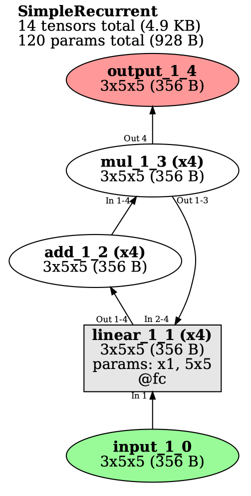
下面是一个非常简单的循环模型的示例;正如您所看到的,您只需像正常定义模型一样将其传入,TorchLens将返回完整的前向传递日志以及可视化结果:
class SimpleRecurrent(nn.Module):
    def __init__(self):
        super().__init__()
        self.fc = nn.Linear(in_features=5, out_features=5)

    def forward(self, x):
        for r in range(4):
            x = self.fc(x)
            x = x + 1
            x = x * 2
        return x


simple_recurrent = SimpleRecurrent()
model_history = tl.log_forward_pass(simple_recurrent, x,
                                    layers_to_save='all',
                                    vis_opt='rolled')
print(model_history['linear_1_1:2'].tensor_contents)  # second pass of first linear layer

'''
tensor([[-0.0690, -1.3957, -0.3231, -0.1980,  0.7197],
        [-0.1083, -1.5051, -0.2570, -0.2024,  0.8248],
        [ 0.1031, -1.4315, -0.5999, -0.4017,  0.7580],
        [-0.0396, -1.3813, -0.3523, -0.2008,  0.6654],
        [ 0.0980, -1.4073, -0.5934, -0.3866,  0.7371],
        [-0.1106, -1.2909, -0.3393, -0.2439,  0.7345]])
'''
这是一个非常复杂的变压器模型(swin_v2_b),其前向传递过程中涉及了1932个操作;我们也可以获取每个操作的保存输出。

2. 安装TorchLens
要安装TorchLens,请先安装graphviz(用于生成网络可视化),然后使用pip安装TorchLens:
sudo apt install graphviz
pip install torchlens
TorchLens与PyTorch的1.8.0及以上版本兼容
3. 如何使用TorchLens
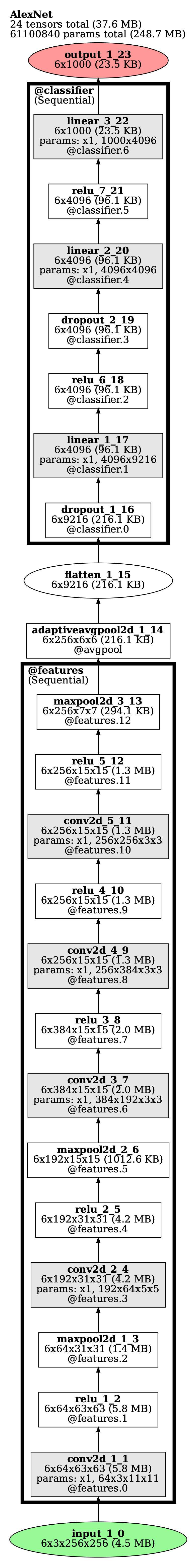
TorchLens的主要功能是log_forward_pass:当在模型和输入上调用时,它会在模型上运行前向传递,并返回一个包含中间层激活和相关元数据的ModelHistory对象,同时还提供了在前向传递过程中发生的每个操作的可视化表示:
import torch
import torchvision
import torchlens as tl

alexnet = torchvision.models.alexnet()
x = torch.rand(1, 3, 224, 224)
model_history = tl.log_forward_pass(alexnet, x, layers_to_save='all', vis_opt='unrolled')
print(model_history)

'''
Log of AlexNet forward pass:
    Model structure: purely feedforward, without branching; 23 total modules.
    24 tensors (4.8 MB) computed in forward pass; 24 tensors (4.8 MB) saved.
    16 parameter operations (61100840 params total; 248.7 MB).
    Random seed: 3210097511
    Time elapsed: 0.288s
    Module Hierarchy:
        features:
            features.0, features.1, features.2, features.3, features.4, features.5, features.6, features.7,
            features.8, features.9, features.10, features.11, features.12
        avgpool
        classifier:
            classifier.0, classifier.1, classifier.2, classifier.3, classifier.4, classifier.5, classifier.6
    Layers:
        0: input_1_0
        1: conv2d_1_1
        2: relu_1_2
        3: maxpool2d_1_3
        4: conv2d_2_4
        5: relu_2_5
        6: maxpool2d_2_6
        7: conv2d_3_7
        8: relu_3_8
        9: conv2d_4_9
        10: relu_4_10
        11: conv2d_5_11
        12: relu_5_12
        13: maxpool2d_3_13
        14: adaptiveavgpool2d_1_14
        15: flatten_1_15
        16: dropout_1_16
        17: linear_1_17
        18: relu_6_18
        19: dropout_2_19
        20: linear_2_20
        21: relu_7_21
        22: linear_3_22
        23: output_1_23
'''
我们通过以下等效的方式从ModelHistory对象中提取有关给定层的信息,包括其激活和有用的元数据:
- 通过层的名称(按照“conv2d_3_7”表示第3个卷积层,总共是第7个层)
- 通过该层作为输出的模块的名称(例如,“features”或“classifier.3”)
- 通过层的序号位置(例如,第2个层为2,倒数第五个为-5;这里输入和输出也被视为层)
要快速确定这些名称,您可以查看图形可视化或打印ModelHistory对象的输出(如上所示)。以下是一些示例,说明如何提取有关特定层的信息,以及如何提取该层的实际激活值:
print(model_history['conv2d_3_7'])  # pulling out layer by its name
# The following commented lines pull out the same layer:
# model_history['conv2d_3'] you can omit the second number (since strictly speaking it's redundant)
# model_history['conv2d_3_7:1'] colon indicates the pass of a layer (here just one)
# model_history['features.6'] can grab a layer by the module for which it is an output
# model_history[7] the 7th layer overall
# model_history[-17] the 17th-to-last layer
'''
Layer conv2d_3_7, operation 8/24:
    Output tensor: shape=(1, 384, 13, 13), dype=torch.float32, size=253.5 KB
        tensor([[ 0.0503, -0.1089, -0.1210, -0.1034, -0.1254],
        [ 0.0789, -0.0752, -0.0581, -0.0372, -0.0181],
        [ 0.0949, -0.0780, -0.0401, -0.0209, -0.0095],
        [ 0.0929, -0.0353, -0.0220, -0.0324, -0.0295],
        [ 0.1100, -0.0337, -0.0330, -0.0479, -0.0235]])...
    Params: Computed from params with shape (384,), (384, 192, 3, 3); 663936 params total (2.5 MB)
    Parent Layers: maxpool2d_2_6
    Child Layers: relu_3_8
    Function: conv2d (gradfunc=ConvolutionBackward0)
    Computed inside module: features.6
    Time elapsed:  5.670E-04s
    Output of modules: features.6
    Output of bottom-level module: features.6
    Lookup keys: -17, 7, conv2d_3_7, conv2d_3_7:1, features.6, features.6:1
'''

# You can pull out the actual output activations from a layer with the tensor_contents field:
print(model_history['conv2d_3_7'].tensor_contents)
'''
tensor([[[[-0.0867, -0.0787, -0.0817,  ..., -0.0820, -0.0655, -0.0195],
          [-0.1213, -0.1130, -0.1386,  ..., -0.1331, -0.1118, -0.0520],
          [-0.0959, -0.0973, -0.1078,  ..., -0.1103, -0.1091, -0.0760],
          ...,
          [-0.0906, -0.1146, -0.1308,  ..., -0.1076, -0.1129, -0.0689],
          [-0.1017, -0.1256, -0.1100,  ..., -0.1160, -0.1035, -0.0801],
          [-0.1006, -0.0941, -0.1204,  ..., -0.1146, -0.1065, -0.0631]]...
'''
如果我们不希望保存所有层的激活值(例如,为了节省内存),您可以在调用log_forward_pass时使用layers_to_save参数指定要保存的层;您可以通过与上述索引方式相同的方式指定层,或者通过传入一个用于筛选层的子字符串(例如,’conv’将提取所有的卷积层)
# Pull out conv2d_3_7, the output of the 'features' module, the fifth-to-last layer, and all linear (i.e., fc) layers:
model_history = tl.log_forward_pass(alexnet, x, vis_opt='unrolled',
                                    layers_to_save=['conv2d_3_7', 'features', -5, 'linear'])
print(model_history.layer_labels)
'''
['conv2d_3_7', 'maxpool2d_3_13', 'linear_1_17', 'dropout_2_19', 'linear_2_20', 'linear_3_22']
'''
4. 其他功能
我们可以使用vis_nesting_depth参数来可视化不同层次的嵌套深度的模型,例如,在这里您可以看到GoogLeNet的一个“inception”模块在不同层次的嵌套深度下的情况: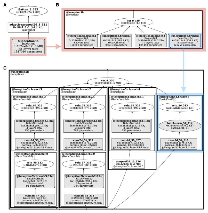
此外这个项目还可以提取反向传播的梯度(可以基于任何中间层计算,而不仅仅是模型的输出),并且可以可视化反向传播的路径(如下图所示的蓝色箭头)。请参考CoLab教程了解如何实现这一功能。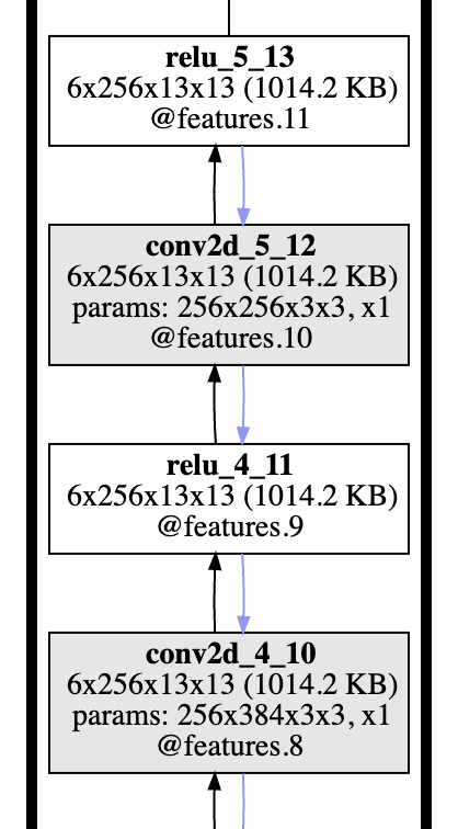


评论(0)
您还未登录,请登录后发表或查看评论